Show code cell content

Hide code cell content

# 1. Import Required Libraries
import numpy as np
from numpy.linalg import svd, norm
import scipy.linalg as sla
from scipy.optimize import least_squares
import matplotlib.pyplot as plt
import random
import warnings

warnings.filterwarnings("ignore")

plt.style.use("seaborn-v0_8")
plt.rcParams["figure.figsize"] = (10, 7)
plt.rcParams["font.size"] = 12

5.3. Direct Linear Transform (DLT)

This notebook demonstrates the Direct Linear Transform (DLT) method for camera calibration, following standard computer vision notation. The DLT provides a linear solution to estimate the camera projection matrix P from known 3D-2D point correspondences.

Learning Objectives: You’ll learn how to estimate a camera’s projection matrix from known 3D-2D point correspondences using the Direct Linear Transform (DLT) algorithm, understand camera matrix decomposition into intrinsic and extrinsic parameters and analyze calibration quality through reprojection error metrics.

5.3.1. Prerequisites

Note

Before reading this chapter you should be comfortable with matrices, vectors, homogeneous transformations, and basic concepts of linear algebra. See chapter Algebra & Calculus for a primer on these foundations.

5.3.2. Camera Projection Model

5.3.2.1. Pinhole Camera Geometry

The pinhole camera model relates 3D world coordinates to 2D image coordinates through perspective projection. Please consult Pinhole Camera Model for detailed information.

We define the homogeneous coordinates for 3D world point \(X\) and image point \(x\):

(5.29)\[ \tilde{X} = [X, Y, Z, 1]^T, \quad \quad \tilde{x} = [u, v, 1]^T \]

now we can write the relation using the projection matrix \(P\)

(5.30)\[\begin{split} \begin{align} s \tilde{x} &= \mathbf{P} \tilde{X} \\ s \begin{bmatrix} u \\ v \\ 1 \end{bmatrix} &= \mathbf{P} \begin{bmatrix} X \\ Y \\ Z \\ 1 \end{bmatrix} \end{align} \end{split}\]

or in proportional (hiding the scale ambiguity) description

(5.31)\[ \tilde{x} \simeq \mathbf{P} \tilde{X} \]

where:

• \((u,v)\) are pixel coordinates in the image

• \((X,Y,Z)\) are 3D world coordinates

• \(s\) is a scale factor (projective depth)

• \(\mathbf{P}\) is the \(3 \times 4\) projection matrix

5.3.2.2. Projection Matrix Decomposition

The projection matrix can be decomposed as:

(5.32)\[ \mathbf{P} = \mathbf{K}[\mathbf{R}|\mathbf{t}] \]

where:

• \(\mathbf{K} \in \mathbb{R}^{3 \times 3}\) is the intrinsic matrix: \(\mathbf{K} = \begin{bmatrix} f_x & \alpha & c_x \\ 0 & f_y & c_y \\ 0 & 0 & 1 \end{bmatrix}\)

  • \(f_x, f_y\): focal lengths in pixels

  • \(c_x, c_y\): principal point coordinates

  • \(\alpha\): skew parameter (usually ≈ 0)

• \(\mathbf{R} \in \mathbb{R}^{3 \times 3}\) is the rotation matrix (world to camera)

• \(\mathbf{t} \in \mathbb{R}^{3 \times 1}\) is the translation vector (camera position in world coordinates)

• \([\mathbf{R}|\mathbf{t}]\) represents the extrinsic parameters (camera pose)

The projection equation becomes:

(5.33)\[\begin{split} s \begin{bmatrix} u \\ v \\ 1 \end{bmatrix} = \mathbf{K} [ \mathbf{R} | \mathbf{t} ] \begin{bmatrix} X \\ Y \\ Z \\ 1 \end{bmatrix} \end{split}\]

5.3.2.3. Degrees of Freedom

The projection matrix \(\mathbf{P}\) has:

• 12 entries total

• 1 scale ambiguity (homogeneous representation)

• 11 degrees of freedom

Therefore, we need ≥ 6 point correspondences (each provides 2 constraints) to solve for \(\mathbf{P}\) up to scale \(s\).

5.3.2.4. Generate Synthetic 3D World Points and Camera Parameters

We create:

• Random 3D points in a cube

• Intrinsic matrix \(\mathbf{K}\) with \(f_x\), \(f_y\), \(\alpha\) (set 0), principal point (\(c_x\), \(c_y\))

• Rotation from Euler angles (\(\mathbf{R_x}\), \(\mathbf{R_y}\), \(\mathbf{R_z}\))

• Translation vector \(t\)

• Camera matrix \(\mathbf{P} = \mathbf{K}[\mathbf{R}|\mathbf{t}]\)

All points are represented in homogeneous coordinates when needed.

def euler_xyz(rx, ry, rz):
    """Compose rotation matrix from Euler angles (radians)."""
    Rx = np.array(
        [[1, 0, 0], [0, np.cos(rx), -np.sin(rx)], [0, np.sin(rx), np.cos(rx)]]
    )
    Ry = np.array(
        [[np.cos(ry), 0, np.sin(ry)], [0, 1, 0], [-np.sin(ry), 0, np.cos(ry)]]
    )
    Rz = np.array(
        [[np.cos(rz), -np.sin(rz), 0], [np.sin(rz), np.cos(rz), 0], [0, 0, 1]]
    )
    return Rz @ Ry @ Rx  # Z-Y-X order


def generate_intrinsics(fx=1200, fy=1180, cx=640, cy=360, alpha=0.0):
    K = np.array([[fx, alpha, cx], [0.0, fy, cy], [0.0, 0.0, 1.0]])
    return K

5.3.2.5. Exercies 1: Create a function to create the projection_matrix

• Fill the given template to construct the projection matrix

• Test it in the following cell

def assemble_projection_matrix(K, R, t):
    """Return 3x4 camera matrix P = K [R|t]."""
    pass

Show code cell content

Hide code cell content

def assemble_projection_matrix(K, R, t):
    """Return 3x4 camera matrix P = K [R|t]."""
    return K @ np.hstack([R, t.reshape(3, 1)])

# Function to generate random 3D scene points
def generate_scene(n_points=40, seed=42, cube_size=2.0):
    rng = np.random.default_rng(seed)
    Xw = rng.uniform(-cube_size, cube_size, (n_points, 3))
    return Xw


# Example camera
rx, ry, rz = np.deg2rad([10, -5, 20])
R_gt = euler_xyz(rx, ry, rz)
t_gt = np.array([0.5, -0.2, 6.0])  # camera looking roughly toward origin
K_gt = generate_intrinsics()
P_gt = assemble_projection_matrix(K_gt, R_gt, t_gt)

X_world = generate_scene(n_points=6, seed=42)
print("Ground truth camera matrix P:\n", P_gt)
print()
print("First 2 world points:\n", X_world[:2])

Ground truth camera matrix P:
 [[ 1.17911984e+03 -3.10543036e+02  6.02361534e+02  4.44000000e+03]
 [ 4.33424078e+02  1.14815901e+03  1.25993858e+02  1.92400000e+03]
 [ 8.71557427e-02  1.72987394e-01  9.81060262e-01  6.00000000e+00]]

First 2 world points:
 [[ 1.09582419 -0.24448624  1.43439168]
 [ 0.78947212 -1.62329061  1.90248941]]

5.3.2.6. Exercies 2: Create a function to project points

• Write a function that calculates the 3D projections.

• It requires the projection matrix \(\mathbf{P}\) and set of 3D points \(X\) as input arguments.

• Run it on the generated 3D world points.

def project_points(P, X):
    """Project (N,3) world points X using camera P (3x4). Return (N,2) image points."""
    pass

Show code cell content

Hide code cell content

def project_points(P, X):
    """Project (N,3) world points X using camera P (3x4). Return (N,2) image points."""
    N = X.shape[0]
    X_h = np.hstack([X, np.ones((N, 1))])  # (N,4)
    x_h = (P @ X_h.T).T  # (N,3)
    x = x_h[:, :2] / x_h[:, 2:3]
    return x, x_h

x_gt, xh_gt = project_points(P_gt, X_world)
print("Sample projected points of the first 2 world points:\n", x_gt[:2])

Sample projected points of the first 2 world points:
 [[894.32457186 308.15506282]
 [917.23973743  83.88349871]]

5.3.3. 4. DLT Algorithm: Linear Solution

The Direct Linear Transform (DLT) method exploits the fundamental property that for any 3D point \(X\) projecting to image point \(x\) equation (5.31) is valid. This means the vectors \(\tilde{x}\) and \(P \tilde{X}\) are parallel (or anti-parallel).

5.3.3.1. Cross Product Property

Note

For a primer on vector cross products, see our Vector Cross Product chapter.

Since parallel vectors have zero cross product:

(5.34)\[ \tilde{x} \times (\mathrm{P} \tilde{X}) = 0 \]

This is the key insight that transforms the projective equation into a linear homogeneous system.

Let’s expand (5.34) systematically:

\[\begin{split} \mathrm{P} = \begin{bmatrix} p_1^T \\ p_2^T \\ p_3^T \end{bmatrix} = \begin{bmatrix} p_{11} & p_{12} & p_{13} & p_{14} \\ p_{21} & p_{22} & p_{23} & p_{24} \\ p_{31} & p_{32} & p_{33} & p_{34} \end{bmatrix} \end{split}\]

The projection gives:

\[\begin{split} \mathrm{P} \tilde{X} = \begin{bmatrix} p_1^T \tilde{X} \\ p_2^T \tilde{X} \\ p_3^T \tilde{X} \end{bmatrix} \end{split}\]

Now equation (5.34) can be written as:

(5.35)\[\begin{split} \begin{bmatrix} u \\ v \\ 1 \end{bmatrix} \times \begin{bmatrix} p_1^T \tilde{X} \\ p_2^T \tilde{X} \\ p_3^T \tilde{X} \end{bmatrix} = \begin{bmatrix} v(p_3^T \tilde{X}) - 1(p_2^T \tilde{X}) \\ 1(p_1^T \tilde{X}) - u(p_3^T \tilde{X}) \\ u(p_2^T \tilde{X}) - v(p_1^T \tilde{X}) \end{bmatrix} = \begin{bmatrix} 0 \\ 0 \\ 0 \end{bmatrix} \end{split}\]

5.3.3.2. Rearranging into Standard DLT Form

Rearranging the first two lines of (5.35) yields two equation. The third one is irrelevant as it is a linear combination of the first two.

Equation 1:

\[p_2^T \tilde{X} - v(p_3^T \tilde{X}) = 0\]

Equation 2:

\[p_1^T \tilde{X} - u(p_3^T \tilde{X}) = 0\]

We want the rewrite the previous equation as a linear system of equations in the standard form of \(\mathrm{A} p = b\), with \(b=0\) and \(p = [p_1^T, p_2^T, p_3^T]^T\) as a 12-element vector, each equation becomes a row in matrix \(A\):

Row 1 (from equation 2):

\[\begin{split} \begin{align} [\tilde{X}^T, 0^T, -u\tilde{X}^T] p &= 0 \\ [X, Y, Z, 1, 0, 0, 0, 0, -uX, -uY, -uZ, -u] p &= 0 \end{align} \end{split}\]

Row 2 (from equation 1):

\[\begin{split} \begin{align} [0^T, \tilde{X}^T, -v\tilde{X}^T] p &= 0 \\ [0, 0, 0, 0, X, Y, Z, 1, -vX, -vY, -vZ, -v] p &= 0 \end{align} \end{split}\]

Essentially we have 2 equations per measurement point and 12 unknowns of the \(\mathrm{P}\) matrix.

The DLT method essentially asks: “What camera matrix makes all observed image rays parallel to their corresponding projected 3D points?”

This cross product formulation is the mathematical foundation that makes camera calibration a linear algebra problem solvable via SVD!

5.3.3.3. Exercise 3: Create a function to create the DLT (or A) matrix

• Use the 3D points and 2D image points as inputs

• For each measurement create 2 rows

def build_dlt_matrix(X, x):
    """Build DLT design matrix A from 3D points X (N,3) and image points x (N,2)."""
    N = X.shape[0]
    A = []
    for i in range(N):
        pass

Show code cell content

Hide code cell content

def build_dlt_matrix(X, x):
    """Build DLT design matrix A from 3D points X (N,3) and image points x (N,2)."""
    N = X.shape[0]
    A = []
    for i in range(N):
        Xx, Yx, Zx = X[i]
        u, v = x[i]
        row1 = [Xx, Yx, Zx, 1, 0, 0, 0, 0, -u * Xx, -u * Yx, -u * Zx, -u]
        row2 = [0, 0, 0, 0, Xx, Yx, Zx, 1, -v * Xx, -v * Yx, -v * Zx, -v]
        A.append(row1)
        A.append(row2)
    return np.array(A)

A = build_dlt_matrix(X_world, x_gt)
print("A shape:", A.shape)
print("First 2 rows:\n", A[:2])

A shape: (12, 12)
First 2 rows:
 [[ 1.09582419e+00 -2.44486241e-01  1.43439168e+00  1.00000000e+00
   0.00000000e+00  0.00000000e+00  0.00000000e+00  0.00000000e+00
  -9.80022503e+02  2.18650053e+02 -1.28281172e+03 -8.94324572e+02]
 [ 0.00000000e+00  0.00000000e+00  0.00000000e+00  0.00000000e+00
   1.09582419e+00 -2.44486241e-01  1.43439168e+00  1.00000000e+00
  -3.37683773e+02  7.53396730e+01 -4.42015058e+02 -3.08155063e+02]]

5.3.3.4. Solve Homogeneous System via SVD

Read the information on Column Space and Null Space to gain information on null spaces. The null space is the solution to the aforementioned equation \(\mathrm{A} p = 0\).

We compute the singular value decomposition (SVD):

(5.36)\[ A = U \Sigma V^T \]

The null space vector p, i.e. the solution of matrix \(A\) (up to scale), is the last column of V corresponding to the smallest singular value.

Connects to earlier rank/null space concepts:

• Expect \(\mathrm{rank}(A) = 11\) (nullity 1) when there are sufficient non-degenerate points (≥6).

def solve_dlt(A, analyze=True):
    """Solve A p = 0 via SVD, return p (length 12)."""

    U, S, Vt = svd(A)
    p = Vt[-1]  # last row of V^T, i.e., last column of V

    if analyze:
        rankA = np.sum(S > 1e-10)
        cond = (
            S[0] / S[-2]
        )  # ignore last singular value which is (near) zero in our dlt case
        print("Design matrix shape:", A.shape)
        print()
        print("Rank(A):", rankA, "Nullity:", A.shape[1] - rankA)
        print()
        print("Singular values:\n", S)
        print()
        print("Condition number:", cond)
        print()
        res = norm(A @ p)
        print("||A p||_2:", res)

    return p


p_est_raw = solve_dlt(A, analyze=True)

Design matrix shape: (12, 12)

Rank(A): 11 Nullity: 1

Singular values:
 [3.85223749e+03 2.84321198e+03 1.14471066e+03 9.91327067e+02
 4.21212466e+00 2.80364060e+00 1.84955587e+00 1.20674556e+00
 6.13219176e-01 3.03575643e-01 2.69256383e-01 3.84821912e-15]

Condition number: 14306.949527170735

||A p||_2: 1.355399879558074e-13

5.3.3.5. Reshape Parameter Vector into Camera Matrix

Reshape p into P_est (3×4). Because the homogeneous system yields scale ambiguity, enforce a scale convention (e.g. \(||P_{est}[2,:]|| = 1\) or divide by last element if sensible).

def vector_to_camera(p):
    P = p.reshape(3, 4)
    # Scale convention: normalize third row norm
    scale = norm(P[2, :])
    P /= scale
    return P


P_est = vector_to_camera(p_est_raw)
print("Estimated camera matrix P_est:\n", P_est)
print("Ground truth (scaled for comparison):\n", P_gt / norm(P_gt[2, :]))

Estimated camera matrix P_est:
 [[-1.93846108e+02  5.10529606e+01 -9.90276262e+01 -7.29931504e+02]
 [-7.12544796e+01 -1.88756179e+02 -2.07132626e+01 -3.16303652e+02]
 [-1.43283158e-02 -2.84389524e-02 -1.61285314e-01 -9.86393924e-01]]
Ground truth (scaled for comparison):
 [[ 1.93846108e+02 -5.10529606e+01  9.90276262e+01  7.29931504e+02]
 [ 7.12544796e+01  1.88756179e+02  2.07132626e+01  3.16303652e+02]
 [ 1.43283158e-02  2.84389524e-02  1.61285314e-01  9.86393924e-01]]

5.3.4. 7. Camera Matrix Decomposition

5.3.4.1. RQ Factorization

The estimated camera matrix can be decomposed in a orthonormal part and upper triangular part which correspond with the extrinsic and intrinsic part. Decomposing can be done using the QR or RQ decomposition methods.

Given \(\mathbf{P} = [\mathbf{M} | \mathbf{m}_4]\) where \(\mathbf{M} = \mathbf{K}\mathbf{R}\) is \(3 \times 3\):

\[\mathbf{M} = \mathbf{K} \mathbf{R}\]

where:

• \(\mathbf{K}\) is upper triangular (intrinsic parameters)

• \(\mathbf{R}\) is orthogonal (rotation matrix)

5.3.4.2. Intrinsic Matrix Structure

\[\begin{split}\mathbf{K} = \begin{bmatrix} f_x & \alpha & c_x \\ 0 & f_y & c_y \\ 0 & 0 & 1 \end{bmatrix}\end{split}\]

• \(f_x, f_y\): focal lengths (pixels)

• \(c_x, c_y\): principal point coordinates

• \(\alpha\): skew parameter (usually ≈ 0)

5.3.4.3. Translation Recovery

Once \(\mathbf{K}\) and \(\mathbf{R}\) are known: $\(\mathbf{t} = \mathbf{K}^{-1} \mathbf{m}_4\)$

Note: Translation is recovered up to scale (fundamental limitation of projective geometry).

def decompose_camera_matrix(P):
    """Decompose camera matrix into K, R, t using RQ on left 3x3."""
    M = P[:, :3]
    K, R = sla.rq(M)  # R is orthogonal, K is upper-triangular
    # Enforce positive diagonal
    T = np.diag(np.sign(np.diag(K)))
    K = K @ T
    R = T @ R
    # Normalize K (K[2,2] should be 1)
    K /= K[2, 2]
    t = np.linalg.inv(K) @ P[:, 3]
    return K, R, t


K_est, R_est, t_est = decompose_camera_matrix(P_est)

print("Estimated K:\n", K_est)
print("Ground truth K:\n", K_gt)
print("\nRotation error (Fro norm):", norm(R_est - R_gt, ord="fro"))
print("Translation est:", t_est)
print("Translation gt:", t_gt)

Estimated K:
 [[1.20000000e+03 3.40178182e-10 6.40000000e+02]
 [0.00000000e+00 1.18000000e+03 3.60000000e+02]
 [0.00000000e+00 0.00000000e+00 1.00000000e+00]]
Ground truth K:
 [[1.20e+03 0.00e+00 6.40e+02]
 [0.00e+00 1.18e+03 3.60e+02]
 [0.00e+00 0.00e+00 1.00e+00]]

Rotation error (Fro norm): 3.4641016151377553
Translation est: [-0.08219949  0.0328798  -0.98639392]
Translation gt: [ 0.5 -0.2  6. ]

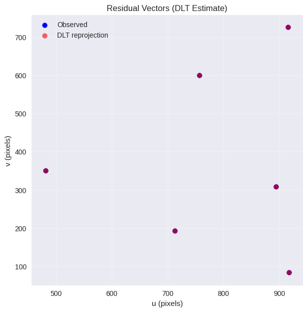
5.3.5. Reprojection Error Evaluation

The reprojection error measures how well our estimated camera matrix P reproduces the observed 2D points from known 3D points.

Definition: For each 3D-2D correspondence \((X_i, x_i)\):

• Project 3D point: \(\hat{x}_i = \text{project}(P, X_i)\)

• Compute Euclidean distance: \(e_i = \|x_i - \hat{x}_i\|_2\)

Geometric Meaning: Reprojection error represents the pixel distance between:

• Observed image points \(x_i\) (ground truth)

• Predicted image points \(\hat{x}_i\) (from estimated camera)

Quality Metrics:

• Mean error: Average distance across all points

• RMS error: \(\sqrt{\frac{1}{n}\sum e_i^2}\) (standard calibration metric)

• Max error: Worst-case correspondence (outlier detection)

We compute mean, RMS, max errors and visualize residual vectors.

def reprojection(P, X):
    x, _ = project_points(P, X)
    return x


def reprojection_error(P, X, x_obs):
    x_est = reprojection(P, X)
    residuals = x_est - x_obs
    errs = np.sqrt(np.sum(residuals**2, axis=1))
    stats = {
        "mean": np.mean(errs),
        "rms": np.sqrt(np.mean(errs**2)),
        "max": np.max(errs),
    }
    return stats, residuals


stats_gt, _ = reprojection_error(P_gt, X_world, x_gt)
stats_est, residuals_est = reprojection_error(P_est, X_world, x_gt)

print("Ground truth reprojection stats (should be near zero):", stats_gt)
print("DLT reprojection stats:", stats_est)

# Plot residuals
plt.figure(figsize=(7, 7))
plt.scatter(x_gt[:, 0], x_gt[:, 1], c="blue", label="Observed")
x_dlt = reprojection(P_est, X_world)
plt.scatter(x_dlt[:, 0], x_dlt[:, 1], c="red", alpha=0.6, label="DLT reprojection")

for i in range(len(x_gt)):
    plt.arrow(
        x_gt[i, 0],
        x_gt[i, 1],
        residuals_est[i, 0],
        residuals_est[i, 1],
        color="green",
        head_width=2.0,
        length_includes_head=True,
        alpha=0.5,
    )

plt.title("Residual Vectors (DLT Estimate)")
plt.xlabel("u (pixels)")
plt.ylabel("v (pixels)")
plt.legend()
plt.grid(alpha=0.3)
plt.show()

Ground truth reprojection stats (should be near zero): {'mean': 0.0, 'rms': 0.0, 'max': 0.0}
DLT reprojection stats: {'mean': 3.89559070460572e-11, 'rms': 4.462257296118922e-11, 'max': 6.488033381345533e-11}

5.3.6. Rank, Null Space, and Conditioning Analysis

We analyze matrix A:

• Rank should be 11 for sufficient non-degenerate points

• Singular spectrum gives conditioning insight

• Null space dimension 1 mirrors earlier column-space-null-space discussions

Large condition numbers indicate sensitivity to noise.

solve_dlt(A, analyze=True)
# solve_dlt(A_norm)

X_world_ = generate_scene(n_points=200, seed=4)
x_gt_, _ = project_points(P_gt, X_world_)
solve_dlt(build_dlt_matrix(X_world_, x_gt_), analyze=True)

Design matrix shape: (12, 12)

Rank(A): 11 Nullity: 1

Singular values:
 [3.85223749e+03 2.84321198e+03 1.14471066e+03 9.91327067e+02
 4.21212466e+00 2.80364060e+00 1.84955587e+00 1.20674556e+00
 6.13219176e-01 3.03575643e-01 2.69256383e-01 3.84821912e-15]

Condition number: 14306.949527170735

||A p||_2: 1.355399879558074e-13
Design matrix shape: (400, 12)

Rank(A): 11 Nullity: 1

Singular values:
 [1.73520571e+04 1.50940812e+04 1.40818549e+04 9.29858004e+03
 1.82332070e+01 1.64449042e+01 1.51086987e+01 1.35289715e+01
 6.44711320e+00 6.11522285e+00 5.16813784e+00 2.69580147e-15]

Condition number: 3357.5066397070864

||A p||_2: 2.1188397530174233e-12

array([-2.27822075e-01,  6.00011605e-02, -1.16384484e-01, -8.57868707e-01,
       -8.37434580e-02, -2.21840019e-01, -2.43437360e-02, -3.71743106e-01,
       -1.68396811e-05, -3.34235297e-05, -1.89554256e-04, -1.15928204e-03])

5.3.7. Degeneracy and Minimal Configuration Tests

DLT for a 3x4 camera requires at least 6 point correspondences (12 equations) but in practice more for stability.

Degenerate cases:

• All points coplanar (world points in a plane) reduce information

• Points arranged on a line

• Insufficient number of points

We demonstrate rank drop and inflated condition numbers.

def degeneracy_demo():
    def make_coplanar_points(n=20, z=0.0, size=4.0):
        rng = np.random.default_rng(1)
        X = rng.uniform(-size, size, (n, 2))
        X3 = np.hstack([X, np.full((n, 1), z)])
        return X3

    X_plane = make_coplanar_points()
    x_plane, _ = project_points(P_gt, X_plane)
    A_plane = build_dlt_matrix(X_plane, x_plane)
    print("Coplanar case:")
    solve_dlt(A_plane)

    X_line = np.array([[i * 0.1, 0, 0] for i in range(20)])
    x_line, _ = project_points(P_gt, X_line)
    A_line = build_dlt_matrix(X_line, x_line)
    print("\nCollinear case:")
    solve_dlt(A_line)

    X_few = X_world[:5]
    x_few, _ = project_points(P_gt, X_few)
    A_few = build_dlt_matrix(X_few, x_few)
    print("\nToo few points (5 world points -> 10 rows):")
    solve_dlt(A_few)


def ill_conditioned_demo():
    print("\n3D very clos:e")
    X_world = generate_scene(n_points=40, seed=4, cube_size=0.01)
    x_gt, _ = project_points(P_gt, X_world)
    solve_dlt(build_dlt_matrix(X_world, x_gt), analyze=True)

    print("\n3D very far apart")
    X_world = generate_scene(n_points=40, seed=4, cube_size=1000.0)
    x_gt, _ = project_points(P_gt, X_world)
    solve_dlt(build_dlt_matrix(X_world, x_gt), analyze=True)


print("\n--- Degeneracy Demo ---")
degeneracy_demo()

print("\n--- Ill-Conditioned Demo ---")
ill_conditioned_demo()

--- Degeneracy Demo ---
Coplanar case:
Design matrix shape: (40, 12)

Rank(A): 8 Nullity: 4

Singular values:
 [1.14838991e+04 8.69010371e+03 3.69218495e+03 9.85399430e+00
 8.86537882e+00 7.62252352e+00 5.89750498e+00 3.04832617e+00
 2.83399619e-13 6.67744231e-14 4.44081103e-18 0.00000000e+00]

Condition number: 2.585991389306951e+21

||A p||_2: 0.0

Collinear case:
Design matrix shape: (40, 12)

Rank(A): 5 Nullity: 7

Singular values:
 [6.82381053e+03 1.64481202e+03 6.44158346e+00 1.79053429e+00
 2.15230664e-01 5.35073516e-14 1.87518157e-14 6.19959988e-16
 1.00898999e-30 2.58571885e-31 0.00000000e+00 0.00000000e+00]

Condition number: inf

||A p||_2: 0.0

Too few points (5 world points -> 10 rows):
Design matrix shape: (10, 12)

Rank(A): 10 Nullity: 2

Singular values:
 [3.74629383e+03 2.84267530e+03 9.91669999e+02 4.98023031e+02
 3.95783162e+00 2.75987750e+00 1.17113458e+00 7.15905038e-01
 2.96993304e-01 1.62792143e-01]

Condition number: 12614.068343471487

||A p||_2: 2.737838346337217e-13

--- Ill-Conditioned Demo ---

3D very clos:e
Design matrix shape: (80, 12)

Rank(A): 11 Nullity: 1

Singular values:
 [5.10011841e+03 3.34694757e+01 2.62754421e+01 2.27855094e+01
 6.32455891e+00 4.16352928e-02 3.30978595e-02 2.85353217e-02
 7.02568928e-05 5.68713023e-05 4.92394028e-05 1.26925102e-15]

Condition number: 103577990.85941572

||A p||_2: 1.635441307864732e-14

3D very far apart
Design matrix shape: (80, 12)

Rank(A): 11 Nullity: 1

Singular values:
 [2.63173530e+08 2.64640628e+07 5.51593155e+06 4.85409881e+04
 4.23719991e+03 4.13017609e+03 3.24558117e+03 3.03838970e+03
 2.75931754e+03 1.66415171e+01 5.90823329e+00 3.53065082e-12]

Condition number: 44543523.8074249

||A p||_2: 6.171896251171249e-09

5.3.8. Noise Sensitivity and Monte Carlo Simulation

We add Gaussian pixel noise and observe:

• Intrinsic parameter errors

• Reprojection errors

• Distributions across trials

This quantifies robustness.

def add_noise(x, sigma=1.0):
    rng = np.random.default_rng()
    return x + rng.normal(0, sigma, x.shape)


def monte_carlo(n_trials=100, noise_sigma=1.0):
    fx_errors, fy_errors, mean_reproj = [], [], []
    for _ in range(n_trials):
        x_noisy = add_noise(x_gt, noise_sigma)
        A_n = build_dlt_matrix(X_world, x_noisy)
        p_raw, _ = solve_dlt(A_n, analyze=False), _
        P_tmp = vector_to_camera(p_raw)
        K_tmp, R_tmp, t_tmp = decompose_camera_matrix(P_tmp)
        stats_tmp, _ = reprojection_error(P_tmp, X_world, x_noisy)
        fx_errors.append(K_tmp[0, 0] - K_gt[0, 0])
        fy_errors.append(K_tmp[1, 1] - K_gt[1, 1])
        mean_reproj.append(stats_tmp["mean"])
    return np.array(fx_errors), np.array(fy_errors), np.array(mean_reproj)


fx_errs, fy_errs, reproj_means = monte_carlo(n_trials=60, noise_sigma=2.5)

plt.figure(figsize=(14, 4))
plt.subplot(1, 3, 1)
plt.hist(fx_errs, bins=15, color="steelblue")
plt.title("fx error distribution")
plt.subplot(1, 3, 2)
plt.hist(fy_errs, bins=15, color="orange")
plt.title("fy error distribution")
plt.subplot(1, 3, 3)
plt.hist(reproj_means, bins=15, color="green")
plt.title("Mean reprojection error")
plt.tight_layout()
plt.show()

print("fx error mean/std:", np.mean(fx_errs), np.std(fx_errs))
print("fy error mean/std:", np.mean(fy_errs), np.std(fy_errs))
print("Mean reprojection error mean/std:", np.mean(reproj_means), np.std(reproj_means))

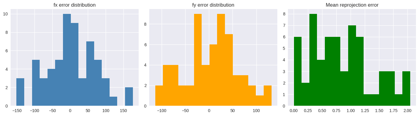
fx error mean/std: 4.015350815073146 70.51873592945384
fy error mean/std: 4.170379344270911 57.39454663339191
Mean reprojection error mean/std: 0.8410928253290628 0.5435490517522839

Show code cell content

Hide code cell content

# # Zhang's Algorithm Implementation
# # Reference: Zhang, Z. (2000). A flexible new technique for camera calibration.
# # IEEE Transactions on Pattern Analysis and Machine Intelligence, 22(11), 1330-1334.


# def compute_homography_dlt(X_plane, x_image):
#     """
#     Compute homography H using DLT from planar points to image points.
#     X_plane: (N, 2) planar coordinates (Z=0 assumed)
#     x_image: (N, 2) image coordinates
#     Returns: H (3x3) homography matrix
#     """
#     N = X_plane.shape[0]
#     if N < 4:
#         raise ValueError("Need at least 4 point correspondences for homography")

#     # Build design matrix for homography DLT
#     A_h = []
#     for i in range(N):
#         X, Y = X_plane[i]  # World plane coordinates
#         u, v = x_image[i]  # Image coordinates

#         # Two rows per correspondence for homography
#         # u = (h1*X + h2*Y + h3) / (h7*X + h8*Y + h9)
#         # v = (h4*X + h5*Y + h6) / (h7*X + h8*Y + h9)
#         # Cross multiply to get linear constraints
#         row1 = [-X, -Y, -1, 0, 0, 0, u * X, u * Y, u]
#         row2 = [0, 0, 0, -X, -Y, -1, v * X, v * Y, v]
#         A_h.append(row1)
#         A_h.append(row2)

#     A_h = np.array(A_h)

#     # Solve via SVD
#     U, S, Vt = svd(A_h)
#     h = Vt[-1]  # Last row of V^T
#     H = h.reshape(3, 3)

#     return H


# def compute_v_ij(H, i, j):
#     """
#     Compute v_ij vector from homography H for Zhang's constraints.
#     Used in absolute conic constraint: v_12^T * omega * v_11 = 0, etc.
#     """
#     h_i = H[:, i]  # i-th column of H
#     h_j = H[:, j]  # j-th column of H

#     # v_ij = [h_i0*h_j0, h_i0*h_j1 + h_i1*h_j0, h_i1*h_j1,
#     #         h_i2*h_j0 + h_i0*h_j2, h_i2*h_j1 + h_i1*h_j2, h_i2*h_j2]
#     v = np.array(
#         [
#             h_i[0] * h_j[0],
#             h_i[0] * h_j[1] + h_i[1] * h_j[0],
#             h_i[1] * h_j[1],
#             h_i[2] * h_j[0] + h_i[0] * h_j[2],
#             h_i[2] * h_j[1] + h_i[1] * h_j[2],
#             h_i[2] * h_j[2],
#         ]
#     )

#     return v


# def estimate_intrinsics_zhang(homographies):
#     """
#     Estimate intrinsic matrix K from multiple homographies using Zhang's method.
#     homographies: list of 3x3 homography matrices
#     Returns: K (3x3) intrinsic matrix
#     """
#     n_views = len(homographies)
#     if n_views < 2:
#         raise ValueError("Zhang's method requires at least 2 views")

#     # Build constraint matrix V for intrinsic parameters
#     V_rows = []

#     for H in homographies:
#         # Two constraints per homography:
#         # 1) h1^T * omega * h2 = 0  (orthogonality)
#         # 2) h1^T * omega * h1 = h2^T * omega * h2  (equal scale)

#         v12 = compute_v_ij(H, 0, 1)  # v_12
#         v11 = compute_v_ij(H, 0, 0)  # v_11
#         v22 = compute_v_ij(H, 1, 1)  # v_22

#         V_rows.append(v12)  # Orthogonality constraint
#         V_rows.append(v11 - v22)  # Equal scale constraint

#     V = np.vstack(V_rows)

#     # Solve V * b = 0 where b = [B11, B12, B22, B13, B23, B33]^T
#     # and B = K^(-T) * K^(-1) is the dual absolute conic
#     U, S, Vt = svd(V)
#     b = Vt[-1]  # Solution vector

#     # Extract elements of symmetric matrix B
#     B11, B12, B22, B13, B23, B33 = b

#     # Compute intrinsic parameters from B matrix
#     # Following Zhang's derivations (Section 3.1)

#     # Principal point
#     v0 = (B12 * B13 - B11 * B23) / (B11 * B22 - B12 * B12)
#     lambda_val = B33 - (B13 * B13 + v0 * (B12 * B13 - B11 * B23)) / B11

#     # Focal lengths
#     fx = np.sqrt(lambda_val / B11)
#     fy = np.sqrt(lambda_val * B11 / (B11 * B22 - B12 * B12))

#     # Skew parameter
#     gamma = -B12 * fx * fx * fy / lambda_val

#     # Principal point x-coordinate
#     u0 = gamma * v0 / fy - B13 * fx * fx / lambda_val

#     # Assemble intrinsic matrix
#     K = np.array([[fx, gamma, u0], [0, fy, v0], [0, 0, 1]])

#     return K


# def compute_extrinsics_zhang(H, K):
#     """
#     Compute extrinsic parameters (R, t) from homography H and intrinsics K.
#     """
#     # H = K * [r1, r2, t] where r1, r2 are first two columns of R

#     # Normalize by intrinsics
#     h1, h2, h3 = H[:, 0], H[:, 1], H[:, 2]

#     K_inv = np.linalg.inv(K)
#     lambda_scale = 1.0 / np.linalg.norm(K_inv @ h1)

#     r1 = lambda_scale * (K_inv @ h1)
#     r2 = lambda_scale * (K_inv @ h2)
#     r3 = np.cross(r1, r2)  # Third column from cross product
#     t = lambda_scale * (K_inv @ h3)

#     # Assemble rotation matrix [r1, r2, r3]
#     R = np.column_stack([r1, r2, r3])

#     # Enforce orthogonality via SVD projection
#     U, S, Vt = svd(R)
#     R_orthogonal = U @ Vt

#     # Ensure proper rotation (det(R) = 1)
#     if np.linalg.det(R_orthogonal) < 0:
#         R_orthogonal[:, -1] *= -1

#     return R_orthogonal, t


# def refine_zhang_parameters(
#     K_init, R_list, t_list, object_points_list, image_points_list
# ):
#     """
#     Refine all parameters using nonlinear optimization (Bundle Adjustment).
#     Minimizes reprojection error across all views.
#     """
#     from scipy.optimize import least_squares

#     n_views = len(R_list)

#     # Parameter vector: [fx, fy, cx, cy, skew, k1, k2] + [rvec1, t1, rvec2, t2, ...]
#     def rodrigues(rvec):
#         """Convert rotation vector to matrix"""
#         theta = np.linalg.norm(rvec)
#         if theta < 1e-12:
#             return np.eye(3)
#         k = rvec / theta
#         K_skew = np.array([[0, -k[2], k[1]], [k[2], 0, -k[0]], [-k[1], k[0], 0]])
#         R = np.eye(3) + np.sin(theta) * K_skew + (1 - np.cos(theta)) * (K_skew @ K_skew)
#         return R

#     def matrix_to_rodrigues(R):
#         """Convert rotation matrix to vector"""
#         trace = np.trace(R)
#         theta = np.arccos(np.clip((trace - 1) / 2, -1, 1))
#         if theta < 1e-12:
#             return np.zeros(3)
#         omega = (
#             theta
#             / (2 * np.sin(theta))
#             * np.array([R[2, 1] - R[1, 2], R[0, 2] - R[2, 0], R[1, 0] - R[0, 1]])
#         )
#         return omega

#     # Initial parameter vector
#     fx, fy = K_init[0, 0], K_init[1, 1]
#     cx, cy = K_init[0, 2], K_init[1, 2]
#     skew = K_init[0, 1]

#     params = [fx, fy, cx, cy, skew, 0.0, 0.0]  # Add distortion coefficients k1, k2

#     for R, t in zip(R_list, t_list):
#         rvec = matrix_to_rodrigues(R)
#         params.extend(rvec)  # 3 rotation parameters
#         params.extend(t)  # 3 translation parameters

#     params = np.array(params)

#     def objective(p):
#         # Unpack parameters
#         fx, fy, cx, cy, skew, k1, k2 = p[:7]

#         K_current = np.array([[fx, skew, cx], [0, fy, cy], [0, 0, 1]])

#         residuals = []
#         param_idx = 7

#         for view_idx in range(n_views):
#             # Extract rotation and translation for this view
#             rvec = p[param_idx : param_idx + 3]
#             t_vec = p[param_idx + 3 : param_idx + 6]
#             param_idx += 6

#             R_current = rodrigues(rvec)

#             # Project points for this view
#             X_3d = object_points_list[view_idx]
#             x_observed = image_points_list[view_idx]

#             # Transform to camera coordinates
#             X_cam = (R_current @ X_3d.T + t_vec.reshape(3, 1)).T

#             # Project to image (with distortion)
#             x_proj = X_cam[:, :2] / X_cam[:, 2:3]

#             # Apply distortion (simple radial model)
#             r2 = x_proj[:, 0] ** 2 + x_proj[:, 1] ** 2
#             distortion = 1 + k1 * r2 + k2 * r2 * r2
#             x_proj *= distortion.reshape(-1, 1)

#             # Apply intrinsics
#             x_proj_h = np.hstack([x_proj, np.ones((len(x_proj), 1))])
#             x_final = (K_current @ x_proj_h.T).T[:, :2]

#             # Residuals
#             residuals.extend((x_final - x_observed).ravel())

#         return np.array(residuals)

#     # Optimize
#     result = least_squares(objective, params, method="trf")

#     # Extract refined parameters
#     p_opt = result.x
#     fx, fy, cx, cy, skew, k1, k2 = p_opt[:7]
#     K_refined = np.array([[fx, skew, cx], [0, fy, cy], [0, 0, 1]])

#     R_refined, t_refined = [], []
#     param_idx = 7
#     for view_idx in range(n_views):
#         rvec = p_opt[param_idx : param_idx + 3]
#         t_vec = p_opt[param_idx + 3 : param_idx + 6]
#         param_idx += 6

#         R_refined.append(rodrigues(rvec))
#         t_refined.append(t_vec)

#     distortion_coeffs = np.array([k1, k2])

#     return K_refined, R_refined, t_refined, distortion_coeffs, result.cost


# def zhang_calibration(object_points_list, image_points_list, refine=True):
#     """
#     Complete Zhang's calibration algorithm.

#     Args:
#         object_points_list: List of (N_i, 3) arrays of 3D points for each view
#         image_points_list: List of (N_i, 2) arrays of corresponding 2D image points
#         refine: Whether to perform nonlinear refinement

#     Returns:
#         K: Intrinsic matrix (3x3)
#         R_list: List of rotation matrices for each view
#         t_list: List of translation vectors for each view
#         distortion_coeffs: Radial distortion coefficients [k1, k2] (if refined)
#         reprojection_error: RMS reprojection error
#     """

#     print("🎯 Zhang's Camera Calibration Algorithm")
#     print("=" * 50)

#     n_views = len(object_points_list)
#     print(f"Processing {n_views} calibration views...")

#     # Step 1: Compute homographies for each view
#     print("1. Computing homographies via DLT...")
#     homographies = []

#     for i, (X_world, x_image) in enumerate(zip(object_points_list, image_points_list)):
#         # Assume planar calibration pattern (Z=0)
#         X_plane = X_world[:, :2]  # Use only X,Y coordinates
#         H = compute_homography_dlt(X_plane, x_image)
#         homographies.append(H)
#         print(
#             f"   View {i+1}: Homography computed (condition: {np.linalg.cond(H):.1e})"
#         )

#     # Step 2: Estimate intrinsic parameters
#     print("2. Estimating intrinsic matrix from homographies...")
#     K_initial = estimate_intrinsics_zhang(homographies)
#     print(f"   Initial intrinsics computed")
#     print(f"   fx={K_initial[0,0]:.1f}, fy={K_initial[1,1]:.1f}")
#     print(f"   cx={K_initial[0,2]:.1f}, cy={K_initial[1,2]:.1f}")

#     # Step 3: Compute extrinsic parameters for each view
#     print("3. Computing extrinsic parameters...")
#     R_list, t_list = [], []

#     for i, H in enumerate(homographies):
#         R, t = compute_extrinsics_zhang(H, K_initial)
#         R_list.append(R)
#         t_list.append(t)
#         print(f"   View {i+1}: Extrinsics computed")

#     # Step 4: Nonlinear refinement (optional)
#     distortion_coeffs = np.zeros(2)
#     if refine:
#         print("4. Nonlinear refinement (Bundle Adjustment)...")
#         K_refined, R_refined, t_refined, distortion_coeffs, final_cost = (
#             refine_zhang_parameters(
#                 K_initial, R_list, t_list, object_points_list, image_points_list
#             )
#         )

#         print(f"   Optimization completed (cost: {final_cost:.6f})")
#         print(
#             f"   Distortion: k1={distortion_coeffs[0]:.6f}, k2={distortion_coeffs[1]:.6f}"
#         )

#         K_final, R_final, t_final = K_refined, R_refined, t_refined
#     else:
#         K_final, R_final, t_final = K_initial, R_list, t_list

#     # Step 5: Compute reprojection error
#     print("5. Evaluating reprojection error...")
#     total_error = 0
#     total_points = 0

#     for i, (X_world, x_image) in enumerate(zip(object_points_list, image_points_list)):
#         # Project using estimated parameters
#         P_estimated = K_final @ np.hstack([R_final[i], t_final[i].reshape(3, 1)])
#         x_reproj, _ = project_points(P_estimated, X_world)

#         error = np.sqrt(np.sum((x_reproj - x_image) ** 2, axis=1))
#         total_error += np.sum(error**2)
#         total_points += len(x_image)

#         print(f"   View {i+1}: RMS error = {np.sqrt(np.mean(error**2)):.3f} pixels")

#     rms_error = np.sqrt(total_error / total_points)
#     print(f"\n📊 Overall RMS reprojection error: {rms_error:.3f} pixels")

#     return K_final, R_final, t_final, distortion_coeffs, rms_error


# # ========== DEMONSTRATION: Zhang vs DLT Comparison ==========


# def run_zhang_vs_dlt_comparison():
#     """Compare Zhang's method with single-view DLT on multi-view data."""

#     print("\n🔍 ZHANG'S METHOD vs DLT COMPARISON")
#     print("=" * 60)

#     # Generate synthetic multi-view calibration data
#     np.random.seed(42)

#     # True camera parameters
#     K_true = np.array([[800, 0, 320], [0, 800, 240], [0, 0, 1]], dtype=float)

#     # Generate multiple checkerboard views with different poses
#     def generate_checkerboard_grid(rows=6, cols=8, square_size=25.0):
#         """Generate checkerboard corner coordinates (planar, Z=0)."""
#         objp = np.zeros((rows * cols, 3), dtype=np.float32)
#         objp[:, :2] = np.mgrid[0:cols, 0:rows].T.reshape(-1, 2)
#         objp *= square_size
#         return objp

#     # Common checkerboard pattern
#     checkerboard_3d = generate_checkerboard_grid()

#     # Different camera poses - ALL cameras positioned in positive Z hemisphere
#     # All cameras looking toward checkerboard at origin (Z=0) from the SAME SIDE (positive Z)
#     poses = [
#         (
#             np.deg2rad([165, 5, 190]),
#             np.array([80, 60, 300]),
#         ),  # View 1: right-top corner
#         (
#             np.deg2rad([170, -15, 188]),
#             np.array([-80, 60, 300]),
#         ),  # View 2: left-top corner
#         (
#             np.deg2rad([175, 15, 185]),
#             np.array([80, -60, 300]),
#         ),  # View 3: right-bottom corner
#         (
#             np.deg2rad([185, -10, 175]),
#             np.array([-80, -60, 300]),
#         ),  # View 4: left-bottom corner
#     ]

#     object_points_multi = []
#     image_points_multi = []

#     print("Generating multi-view synthetic data...")
#     for i, (angles, translation) in enumerate(poses):
#         # Create rotation matrix from Euler angles
#         rx, ry, rz = angles
#         R_true = euler_xyz(rx, ry, rz)
#         t_true = translation

#         # Project checkerboard to image
#         P_true = K_true @ np.hstack([R_true, t_true.reshape(3, 1)])
#         x_clean, _ = project_points(P_true, checkerboard_3d)

#         # Add realistic noise
#         noise = np.random.normal(0, 0.3, x_clean.shape)  # 0.3 pixel std
#         x_noisy = x_clean + noise

#         object_points_multi.append(checkerboard_3d)
#         image_points_multi.append(x_noisy)
#         print(f"   View {i+1}: {len(checkerboard_3d)} points projected")

#     # Method 1: Zhang's Algorithm (multi-view)
#     print(f"\n🎯 Applying Zhang's Algorithm ({len(poses)} views)...")
#     K_zhang, R_zhang, t_zhang, distortion, rms_zhang = zhang_calibration(
#         object_points_multi, image_points_multi, refine=False
#     )

#     # # Method 2: Single-view DLT (using first view only)
#     # print(f"\n⚡ Applying DLT (single view)...")
#     # X_single = object_points_multi[0]
#     # x_single = image_points_multi[0]

#     # P_dlt, cond_dlt = dlt_camera_calibration(X_single, x_single, normalize=True)
#     # K_dlt, R_dlt, t_dlt = decompose_camera_matrix(P_dlt)
#     # rms_dlt = reprojection_error(P_dlt, X_single, x_single)

#     # Comparison Results
#     print(f"\n📊 CALIBRATION RESULTS COMPARISON")
#     print("=" * 60)

#     def parameter_error(K_est, K_true):
#         """Compute relative parameter errors."""
#         fx_err = abs(K_est[0, 0] - K_true[0, 0]) / K_true[0, 0] * 100
#         fy_err = abs(K_est[1, 1] - K_true[1, 1]) / K_true[1, 1] * 100
#         cx_err = abs(K_est[0, 2] - K_true[0, 2]) / K_true[0, 2] * 100
#         cy_err = abs(K_est[1, 2] - K_true[1, 2]) / K_true[1, 2] * 100
#         return fx_err, fy_err, cx_err, cy_err

#     zhang_errors = parameter_error(K_zhang, K_true)
#     # dlt_errors = parameter_error(K_dlt, K_true)

#     # print(
#     #     f"Method                 | RMS Error | fx Error | fy Error | cx Error | cy Error"
#     # )
#     # print(
#     #     f"---------------------- | --------- | -------- | -------- | -------- | --------"
#     # )
#     # print(
#     #     f"Zhang ({len(poses)} views)        | {rms_zhang:8.3f} | {zhang_errors[0]:7.2f}% | {zhang_errors[1]:7.2f}% | {zhang_errors[2]:7.2f}% | {zhang_errors[3]:7.2f}%"
#     # )
#     # print(
#     #     f"DLT (1 view)           | {rms_dlt:8.3f} | {dlt_errors[0]:7.2f}% | {dlt_errors[1]:7.2f}% | {dlt_errors[2]:7.2f}% | {dlt_errors[3]:7.2f}%"
#     # )

#     # print(f"\nTrue Intrinsics:")
#     # print(K_true)
#     # print(f"\nZhang's Estimate:")
#     # print(K_zhang)
#     # print(f"\nDLT Estimate:")
#     # print(K_dlt)

#     # Visualization
#     fig, axes = plt.subplots(1, 3, figsize=(18, 5))

#     # Plot 1: Multi-view setup
#     ax1 = fig.add_subplot(131, projection="3d")
#     colors = ["red", "blue", "green", "orange"]

#     for i, (X_obj, color) in enumerate(zip(object_points_multi, colors)):
#         ax1.scatter(
#             X_obj[:, 0],
#             X_obj[:, 1],
#             X_obj[:, 2],
#             c=color,
#             s=30,
#             alpha=0.7,
#             label=f"View {i+1}",
#         )

#     ax1.set_xlabel("X (mm)")
#     ax1.set_ylabel("Y (mm)")
#     ax1.set_zlabel("Z (mm)")
#     ax1.set_title("Multi-View Calibration Setup")
#     ax1.legend()

#     # Plot 2: Parameter accuracy comparison
#     ax2 = axes[1]
#     params = ["fx", "fy", "cx", "cy"]
#     zhang_vals = [zhang_errors[i] for i in range(4)]
#     # dlt_vals = [dlt_errors[i] for i in range(4)]

#     x_pos = np.arange(len(params))
#     width = 0.35

#     ax2.bar(
#         x_pos - width / 2,
#         zhang_vals,
#         width,
#         label="Zhang",
#         color="steelblue",
#         alpha=0.8,
#     )
#     # ax2.bar(x_pos + width / 2, dlt_vals, width, label="DLT", color="orange", alpha=0.8)

#     ax2.set_xlabel("Parameters")
#     ax2.set_ylabel("Relative Error (%)")
#     ax2.set_title("Parameter Estimation Accuracy")
#     ax2.set_xticks(x_pos)
#     ax2.set_xticklabels(params)
#     ax2.legend()
#     ax2.grid(True, alpha=0.3)

#     # # Plot 3: Reprojection error comparison
#     # ax3 = axes[2]
#     # methods = ["Zhang\n(Multi-view)", "DLT\n(Single-view)"]
#     # rms_values = [rms_zhang, rms_dlt]
#     # colors_bar = ["steelblue", "orange"]

#     # bars = ax3.bar(methods, rms_values, color=colors_bar, alpha=0.8)
#     # ax3.set_ylabel("RMS Reprojection Error (pixels)")
#     # ax3.set_title("Reprojection Error Comparison")
#     # ax3.grid(True, alpha=0.3)

#     # # Add value labels on bars
#     # for bar, val in zip(bars, rms_values):
#     #     ax3.text(
#     #         bar.get_x() + bar.get_width() / 2,
#     #         bar.get_height() + 0.001,
#     #         f"{val:.3f}",
#     #         ha="center",
#     #         va="bottom",
#     #         fontweight="bold",
#     #     )

#     plt.tight_layout()
#     plt.show()

#     return {
#         "zhang": {"K": K_zhang, "rms": rms_zhang, "distortion": distortion},
#         # "dlt": {"K": K_dlt, "rms": rms_dlt},
#         "true": {"K": K_true},
#     }

# from DLT_utils import dlt_camera_calibration

# # Run the demonstration
# comparison_results = run_zhang_vs_dlt_comparison()