Column Space and Null Space

6.4. Column Space and Null Space#

In this notebook, we’ll explore two fundamental concepts in linear algebra: the column space and null space of a matrix. These spaces provide crucial insights into the behavior of linear transformations and systems of linear equations.

6.4.1. Learning Objectives#

By the end of this notebook, you will:

Understand the definitions of column space and null space
Grasp the concepts of matrix rank and inverse matrices
Visualize these spaces geometrically in 2D and 3D
Explore the relationships between all these fundamental concepts
Apply these concepts to solve practical problems

6.4.2. Prerequisites#

Basic understanding of vectors and matrices
Familiarity with linear combinations and spans
Knowledge of matrix multiplication

6.4.3. Reference Material#

This notebook is inspired by and complements the excellent 3Blue1Brown video series on linear algebra:

“Inverse matrices, column space and null space | Chapter 7, Essence of linear algebra”
🎥 Watch on YouTube
Key timestamps:
- 0:00 - Introduction to inverse matrices
- 2:30 - Geometric interpretation of matrix inverse
- 5:45 - Connection to determinants
- 8:20 - Column space and rank
- 11:30 - Null space and its relationship to rank

6.4.4. Matrix Rank: The Foundation Concept#

6.4.4.1. Definition#

The rank of a matrix is one of the most fundamental concepts in linear algebra. It tells us about the “effective dimensionality” of the linear transformation represented by the matrix.

Formal Definition: The rank of an $m \times n$ matrix $A$ is the maximum number of linearly independent column vectors in $A$. Equivalently:

Rank = dimension of the column space
Rank = dimension of the row space
Rank = number of pivot positions after row reduction
Rank = number of non-zero singular values

6.4.4.2. Key Properties#

Range: $0 \leq \text{rank}(A) \leq \min(m,n)$
Full Rank: If $\text{rank}(A) = \min(m,n)$, the matrix has full rank
Rank-Nullity Theorem: $\text{rank}(A) + \text{nullity}(A) = n$
Invariance: Rank is preserved under elementary row operations

6.4.4.3. Geometric Interpretation#

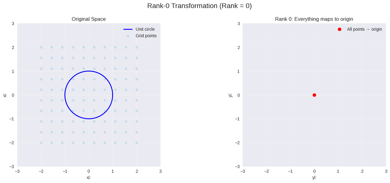
Rank 0: Zero matrix (maps everything to origin)
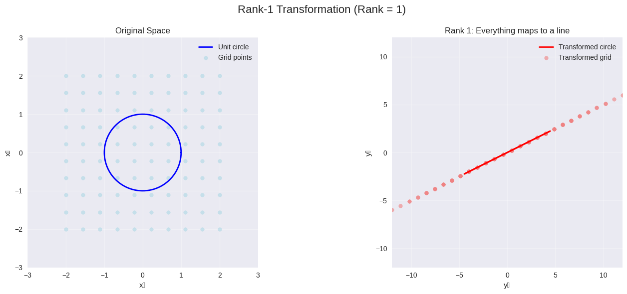
Rank 1: Maps all vectors to a line through the origin
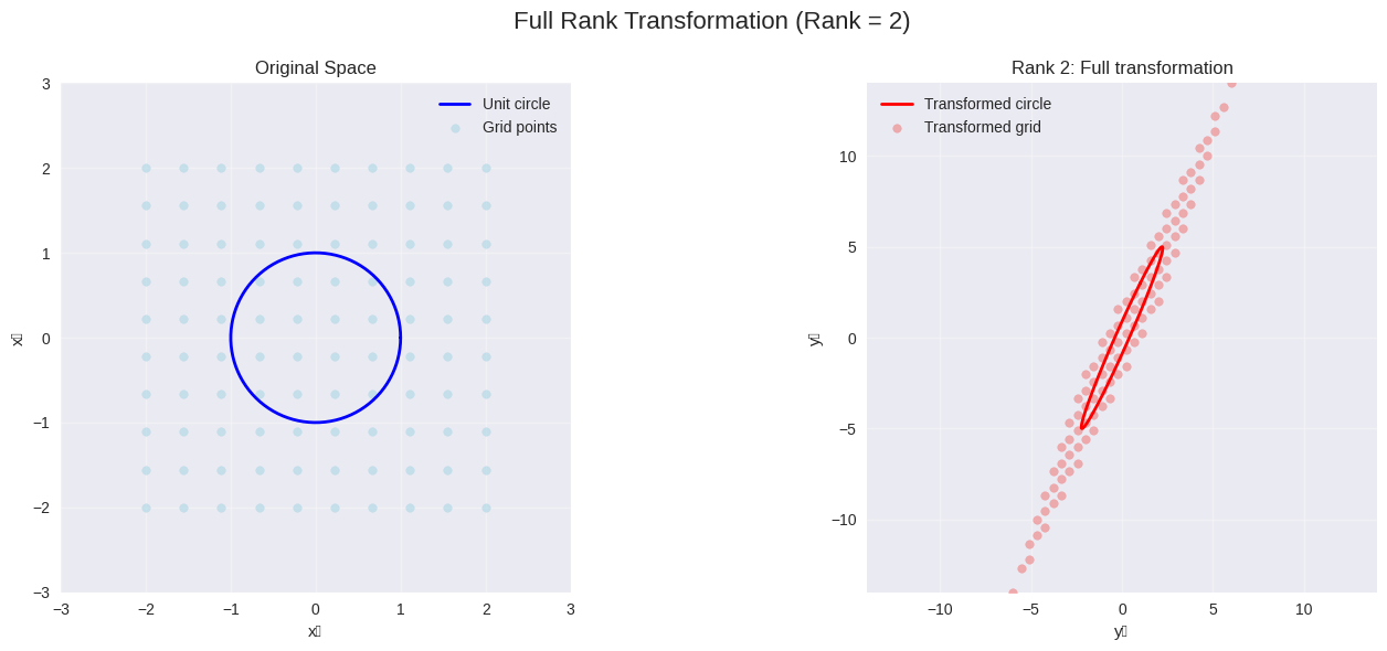
Rank 2: Maps all vectors to a plane through the origin
Full Rank: Preserves dimensionality (invertible if square)

def analyze_rank(A, title="Matrix Rank Analysis"):
    """
    Comprehensive rank analysis
    """
    print(f"{title}")
    print("=" * 50)
    print(f"Matrix A:")
    print(A)

    # Basic properties
    m, n = A.shape
    rank = np.linalg.matrix_rank(A)
    det_A = np.linalg.det(A) if m == n else "N/A (non-square)"

    print(f"\nShape: {m}×{n}")
    print(f"Rank: {rank}")
    print(f"Determinant: {det_A}")
    print(f"Full rank? {'Yes' if rank == min(m,n) else 'No'}")

    # Linear independence analysis
    print(f"\nColumn Analysis:")
    for i in range(n):
        col = A[:, i]
        print(f"  Column {i+1}: {col}")

    if rank < n:
        print(f"  → Columns are linearly DEPENDENT")
        print(f"  → {n - rank} redundant column(s)")
    else:
        print(f"  → Columns are linearly INDEPENDENT")

    # Geometric interpretation
    print(f"\nGeometric Interpretation:")
    if rank == 0:
        print("  → Zero transformation (everything maps to origin)")
    elif rank == 1:
        print("  → All vectors map to a LINE through origin")
    elif rank == 2:
        print("  → All vectors map to a PLANE through origin")
    elif rank == min(m, n):
        print("  → Full-rank transformation (preserves dimension)")

    # Invertibility (for square matrices)
    if m == n:
        is_invertible = rank == n
        print(f"\nInvertibility:")
        print(f"  → {'INVERTIBLE' if is_invertible else 'NOT INVERTIBLE'}")
        if is_invertible:
            print("  → Has unique solution to Ax = b for any b")
        else:
            print("  → Some equations Ax = b have no solution")

# Rank 2 (full rank)
A_rank2 = np.array([[1, 2], [3, 4]])
analyze_rank(A_rank2, "Example 1: Full Rank 2×2 Matrix")

print("\n" + "=" * 60 + "\n")

# Rank 1 (rank deficient)
A_rank1 = np.array([[2, 4], [1, 2]])
analyze_rank(A_rank1, "Example 2: Rank-1 2×2 Matrix")

print("\n" + "=" * 60 + "\n")

# Rank 2 in 3×3 (rank deficient)
A_rank2_3x3 = np.array([[1, 2, 3], [4, 5, 6], [5, 7, 9]])  # Row 3 = Row 1 + Row 2
analyze_rank(A_rank2_3x3, "Example 3: Rank-2 3×3 Matrix")

Example 1: Full Rank 2×2 Matrix
==================================================
Matrix A:
[[1 2]
 [3 4]]

Shape: 2×2
Rank: 2
Determinant: -2.0000000000000004
Full rank? Yes

Column Analysis:
  Column 1: [1 3]
  Column 2: [2 4]
  → Columns are linearly INDEPENDENT

Geometric Interpretation:
  → All vectors map to a PLANE through origin

Invertibility:
  → INVERTIBLE
  → Has unique solution to Ax = b for any b

============================================================

Example 2: Rank-1 2×2 Matrix
==================================================
Matrix A:
[[2 4]
 [1 2]]

Shape: 2×2
Rank: 1
Determinant: 0.0
Full rank? No

Column Analysis:
  Column 1: [2 1]
  Column 2: [4 2]
  → Columns are linearly DEPENDENT
  → 1 redundant column(s)

Geometric Interpretation:
  → All vectors map to a LINE through origin

Invertibility:
  → NOT INVERTIBLE
  → Some equations Ax = b have no solution

============================================================

Example 3: Rank-2 3×3 Matrix
==================================================
Matrix A:
[[1 2 3]
 [4 5 6]
 [5 7 9]]

Shape: 3×3
Rank: 2
Determinant: 3.996802888650562e-15
Full rank? No

Column Analysis:
  Column 1: [1 4 5]
  Column 2: [2 5 7]
  Column 3: [3 6 9]
  → Columns are linearly DEPENDENT
  → 1 redundant column(s)

Geometric Interpretation:
  → All vectors map to a PLANE through origin

Invertibility:
  → NOT INVERTIBLE
  → Some equations Ax = b have no solution

Show code cell content

Hide code cell content

def visualize_rank_transformation(A, title="Rank Visualization"):
    """
    Show how different ranks affect transformations
    """
    rank = np.linalg.matrix_rank(A)

    if A.shape != (2, 2):
        print("This visualization is for 2×2 matrices only")
        return

    # Create unit circle and grid
    theta = np.linspace(0, 2 * np.pi, 100)
    unit_circle = np.array([np.cos(theta), np.sin(theta)])

    # Create grid of points
    x = np.linspace(-2, 2, 10)
    y = np.linspace(-2, 2, 10)
    X, Y = np.meshgrid(x, y)
    grid_points = np.vstack([X.flatten(), Y.flatten()])

    # Transform through matrix A
    transformed_circle = A @ unit_circle
    transformed_grid = A @ grid_points

    # Create visualization
    fig, (ax1, ax2) = plt.subplots(1, 2, figsize=(15, 6))

    # Original space
    ax1.plot(unit_circle[0], unit_circle[1], "b-", linewidth=2, label="Unit circle")
    ax1.scatter(
        grid_points[0],
        grid_points[1],
        c="lightblue",
        alpha=0.6,
        s=30,
        label="Grid points",
    )
    ax1.set_xlim(-3, 3)
    ax1.set_ylim(-3, 3)
    ax1.set_xlabel("x₁")
    ax1.set_ylabel("x₂")
    ax1.set_title("Original Space")
    ax1.grid(True, alpha=0.3)
    ax1.legend()
    ax1.set_aspect("equal")

    # Transformed space
    if rank == 0:
        ax2.plot(0, 0, "ro", markersize=8, label="All points → origin")
        ax2.set_title("Rank 0: Everything maps to origin")
    elif rank == 1:
        ax2.plot(
            transformed_circle[0],
            transformed_circle[1],
            "r-",
            linewidth=2,
            label="Transformed circle",
        )
        ax2.scatter(
            transformed_grid[0],
            transformed_grid[1],
            c="lightcoral",
            alpha=0.6,
            s=30,
            label="Transformed grid",
        )
        ax2.set_title("Rank 1: Everything maps to a line")
    else:  # rank == 2
        ax2.plot(
            transformed_circle[0],
            transformed_circle[1],
            "r-",
            linewidth=2,
            label="Transformed circle",
        )
        ax2.scatter(
            transformed_grid[0],
            transformed_grid[1],
            c="lightcoral",
            alpha=0.6,
            s=30,
            label="Transformed grid",
        )
        ax2.set_title("Rank 2: Full transformation")

    ax2.set_xlabel("y₁")
    ax2.set_ylabel("y₂")
    ax2.grid(True, alpha=0.3)
    ax2.legend()
    ax2.set_aspect("equal")

    # Set equal scales for comparison
    max_val = max(
        np.max(np.abs(transformed_circle)), np.max(np.abs(transformed_grid)), 3
    )
    ax2.set_xlim(-max_val, max_val)
    ax2.set_ylim(-max_val, max_val)

    plt.suptitle(f"{title} (Rank = {rank})", fontsize=16)
    plt.tight_layout()
    plt.show()

# Visualize different ranks
visualize_rank_transformation(A_rank2, "Full Rank Transformation")
visualize_rank_transformation(A_rank1, "Rank-1 Transformation")

# Zero matrix example
A_rank0 = np.array([[0, 0], [0, 0]])
visualize_rank_transformation(A_rank0, "Rank-0 Transformation")

../_images/dc40d4a6ce4fda64b62cb29444576391f8f4e8bcc11193075ca521ea4b24abde.png

../_images/99f38ab3170236283692977b8386faf54de7d8816125264bbe7ec103f10e2097.png

../_images/6fa571b5fe0d189b93e17d6c5f2066bcb2a6d4f7d50453675a084df5b6b78f36.png

6.4.5. Inverse Matrices: Undoing Transformations#

6.4.5.1. Definition#

For a square matrix $A$, the inverse matrix $A^{-1}$ (if it exists) is the unique matrix such that:

\[A A^{-1} = A^{-1} A = I\]

where $I$ is the identity matrix.

6.4.5.2. Key Properties#

Existence: $A^{-1}$ exists if and only if $A$ has full rank (i.e., $\det(A) \neq 0$)
Uniqueness: If the inverse exists, it is unique
Geometric Meaning: $A^{-1}$ “undoes” the transformation of $A$
Computational: For 2×2 matrices: $A^{-1} = \frac{1}{\det(A)} \begin{pmatrix} d & -b \\ -c & a \end{pmatrix}$ where $A = \begin{pmatrix} a & b \\ c & d \end{pmatrix}$

6.4.5.3. When Does an Inverse NOT Exist?#

A matrix is not invertible (singular) when:

Its determinant is zero
Its columns are linearly dependent
It has rank less than its size
Its null space is non-trivial
It maps some non-zero vector to zero

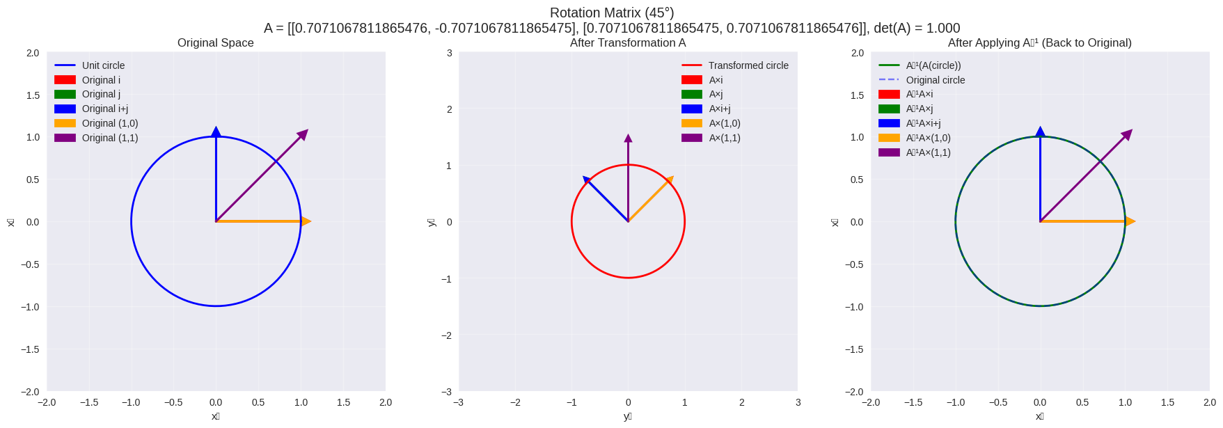
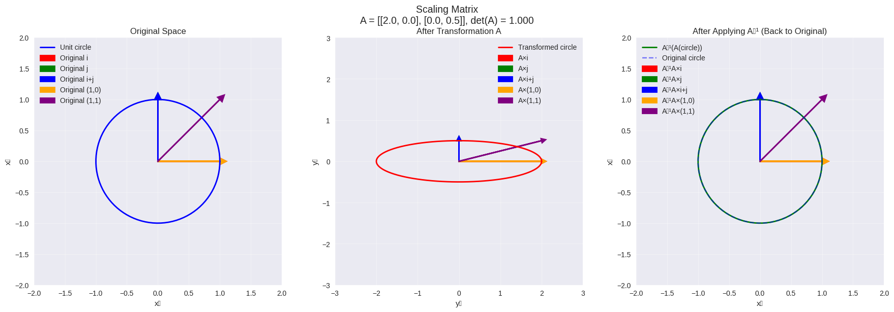
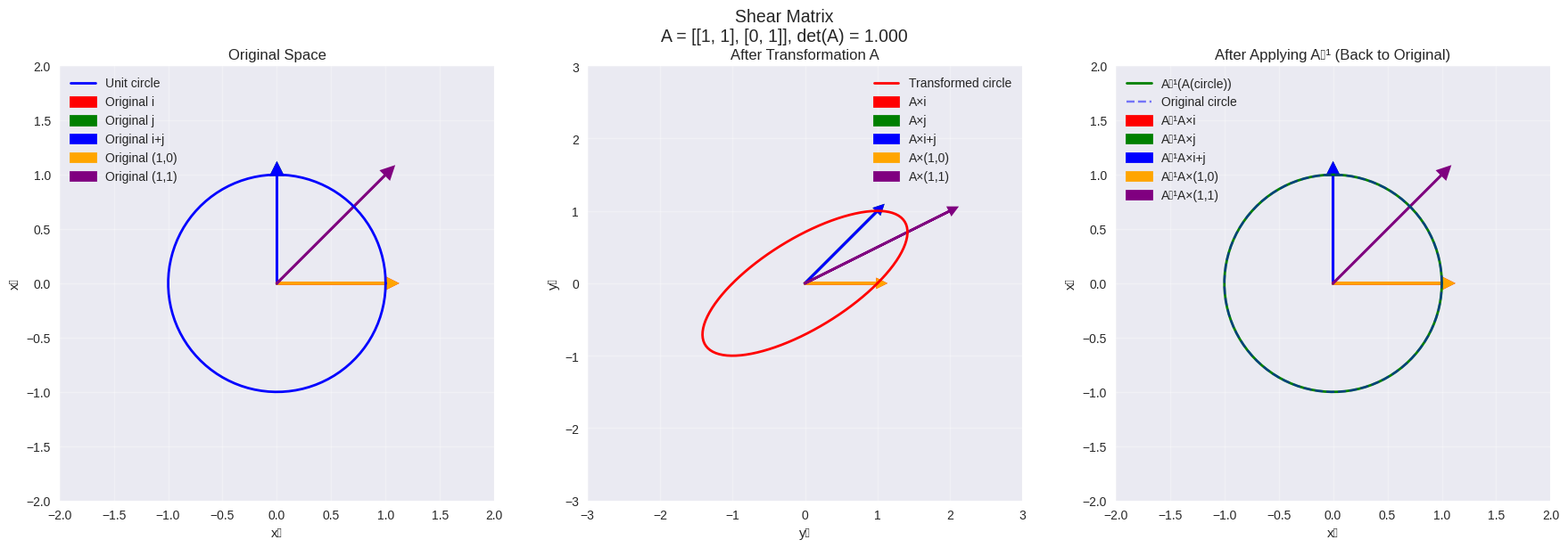
6.4.5.4. Geometric Interpretation#

Think of matrix multiplication as a geometric transformation:

$A$ transforms vectors in some way (rotate, scale, shear)
$A^{-1}$ performs the exact opposite transformation
If $A$ “squashes” space (reduces rank), it cannot be undone → no inverse

def analyze_inverse_matrix(A, title="Inverse Matrix Analysis"):
    """
    Comprehensive analysis of matrix invertibility
    """
    print(f"{title}")
    print("=" * 50)
    print(f"Matrix A:")
    print(A)

    if A.shape[0] != A.shape[1]:
        print("Matrix is not square - inverse doesn't exist!")
        return

    n = A.shape[0]
    det_A = np.linalg.det(A)
    rank_A = np.linalg.matrix_rank(A)

    print(f"Determinant: {det_A:.6f}")
    print(f"Rank: {rank_A}")
    print(f"Full rank? {'Yes' if rank_A == n else 'No'}")

    # Check invertibility
    is_invertible = abs(det_A) > 1e-10

    if is_invertible:
        print(f"\n✅ MATRIX IS INVERTIBLE")
        A_inv = np.linalg.inv(A)
        print(f"Inverse A⁻¹:")
        print(A_inv)

        # Verify the inverse
        print(f"\nVerification:")
        AA_inv = A @ A_inv
        A_inv_A = A_inv @ A
        print(f"A × A⁻¹ =")
        print(AA_inv)
        print(f"A⁻¹ × A =")
        print(A_inv_A)

        # Check how close to identity
        I = np.eye(n)
        error1 = np.linalg.norm(AA_inv - I)
        error2 = np.linalg.norm(A_inv_A - I)
        print(f"Error in A×A⁻¹: {error1:.2e}")
        print(f"Error in A⁻¹×A: {error2:.2e}")

        return A_inv
    else:
        print(f"\n❌ MATRIX IS NOT INVERTIBLE (SINGULAR)")
        print(f"Reasons:")
        print(f"  • Determinant is zero")
        print(f"  • Rank ({rank_A}) < size ({n})")
        print(f"  • Columns are linearly dependent")

        # Show null space
        null_A = null_space(A)
        if null_A.shape[1] > 0:
            print(f"  • Non-trivial null space (dimension {null_A.shape[1]}):")
            for i, vec in enumerate(null_A.T):
                print(f"    Null vector {i+1}: {vec}")
                print(f"    Verification A×v = {A @ vec}")

        return None


# Examples of invertible and non-invertible matrices
print("🔄 INVERSE MATRIX EXAMPLES\n")

# Invertible matrix
A_invertible = np.array([[2, 1], [1, 1]])
A_inv = analyze_inverse_matrix(A_invertible, "Example 1: Invertible Matrix")

print("\n" + "=" * 60 + "\n")

# Non-invertible matrix
A_singular = np.array([[2, 4], [1, 2]])
analyze_inverse_matrix(A_singular, "Example 2: Singular (Non-invertible) Matrix")

print("\n" + "=" * 60 + "\n")

# 3×3 examples
A_3x3_inv = np.array([[1, 2, 0], [0, 1, 1], [1, 0, 1]])
analyze_inverse_matrix(A_3x3_inv, "Example 3: 3×3 Invertible Matrix")

🔄 INVERSE MATRIX EXAMPLES

Example 1: Invertible Matrix
==================================================
Matrix A:
[[2 1]
 [1 1]]
Determinant: 1.000000
Rank: 2
Full rank? Yes

✅ MATRIX IS INVERTIBLE
Inverse A⁻¹:
[[ 1. -1.]
 [-1.  2.]]

Verification:
A × A⁻¹ =
[[1. 0.]
 [0. 1.]]
A⁻¹ × A =
[[1. 0.]
 [0. 1.]]
Error in A×A⁻¹: 0.00e+00
Error in A⁻¹×A: 0.00e+00

============================================================

Example 2: Singular (Non-invertible) Matrix
==================================================
Matrix A:
[[2 4]
 [1 2]]
Determinant: 0.000000
Rank: 1
Full rank? No

❌ MATRIX IS NOT INVERTIBLE (SINGULAR)
Reasons:
  • Determinant is zero
  • Rank (1) < size (2)
  • Columns are linearly dependent
  • Non-trivial null space (dimension 1):
    Null vector 1: [ 0.89442719 -0.4472136 ]
    Verification A×v = [0. 0.]

============================================================

Example 3: 3×3 Invertible Matrix
==================================================
Matrix A:
[[1 2 0]
 [0 1 1]
 [1 0 1]]
Determinant: 3.000000
Rank: 3
Full rank? Yes

✅ MATRIX IS INVERTIBLE
Inverse A⁻¹:
[[ 0.33333333 -0.66666667  0.66666667]
 [ 0.33333333  0.33333333 -0.33333333]
 [-0.33333333  0.66666667  0.33333333]]

Verification:
A × A⁻¹ =
[[ 1.00000000e+00  0.00000000e+00  0.00000000e+00]
 [ 5.55111512e-17  1.00000000e+00 -5.55111512e-17]
 [-5.55111512e-17  0.00000000e+00  1.00000000e+00]]
A⁻¹ × A =
[[ 1.00000000e+00 -1.11022302e-16  1.11022302e-16]
 [ 0.00000000e+00  1.00000000e+00 -5.55111512e-17]
 [ 0.00000000e+00  0.00000000e+00  1.00000000e+00]]
Error in A×A⁻¹: 9.61e-17
Error in A⁻¹×A: 1.67e-16

array([[ 0.33333333, -0.66666667,  0.66666667],
       [ 0.33333333,  0.33333333, -0.33333333],
       [-0.33333333,  0.66666667,  0.33333333]])

Show code cell content

Hide code cell content

def visualize_inverse_transformation(A, title="Inverse Transformation Visualization"):
    """
    Show original transformation and its inverse
    """
    if A.shape != (2, 2):
        print("This visualization is for 2×2 matrices only")
        return

    det_A = np.linalg.det(A)
    if abs(det_A) < 1e-10:
        print(f"Matrix is singular (det = {det_A:.2e}) - no inverse exists!")
        return

    A_inv = np.linalg.inv(A)

    # Create test vectors
    test_vectors = np.array(
        [[1, 0, 0, 1, 1], [0, 1, 1, 0, 1]]
    )  # i, j, i+j, basis vectors

    # Apply transformations
    transformed = A @ test_vectors
    double_transformed = A_inv @ transformed  # Should get back original

    # Create unit circle for visualization
    theta = np.linspace(0, 2 * np.pi, 100)
    unit_circle = np.array([np.cos(theta), np.sin(theta)])
    circle_A = A @ unit_circle
    circle_back = A_inv @ circle_A  # Should be back to unit circle

    # Create 3 subplots
    fig, (ax1, ax2, ax3) = plt.subplots(1, 3, figsize=(18, 6))

    # Plot 1: Original space
    ax1.plot(unit_circle[0], unit_circle[1], "b-", linewidth=2, label="Unit circle")
    colors = ["red", "green", "blue", "orange", "purple"]
    labels = ["i", "j", "i+j", "(1,0)", "(1,1)"]

    for i, (vec, color, label) in enumerate(zip(test_vectors.T, colors, labels)):
        ax1.arrow(
            0,
            0,
            vec[0],
            vec[1],
            head_width=0.1,
            head_length=0.1,
            fc=color,
            ec=color,
            linewidth=2,
            label=f"Original {label}",
        )

    ax1.set_xlim(-2, 2)
    ax1.set_ylim(-2, 2)
    ax1.set_xlabel("x₁")
    ax1.set_ylabel("x₂")
    ax1.set_title("Original Space")
    ax1.grid(True, alpha=0.3)
    ax1.legend()
    ax1.set_aspect("equal")

    # Plot 2: After transformation A
    ax2.plot(circle_A[0], circle_A[1], "r-", linewidth=2, label="Transformed circle")

    for i, (vec, color, label) in enumerate(zip(transformed.T, colors, labels)):
        ax2.arrow(
            0,
            0,
            vec[0],
            vec[1],
            head_width=0.1,
            head_length=0.1,
            fc=color,
            ec=color,
            linewidth=2,
            label=f"A×{label}",
        )

    max_val = max(np.max(np.abs(circle_A)), 3)
    ax2.set_xlim(-max_val, max_val)
    ax2.set_ylim(-max_val, max_val)
    ax2.set_xlabel("y₁")
    ax2.set_ylabel("y₂")
    ax2.set_title("After Transformation A")
    ax2.grid(True, alpha=0.3)
    ax2.legend()
    ax2.set_aspect("equal")

    # Plot 3: After applying inverse (should be back to original)
    ax3.plot(circle_back[0], circle_back[1], "g-", linewidth=2, label="A⁻¹(A(circle))")
    ax3.plot(unit_circle[0], unit_circle[1], "b--", alpha=0.5, label="Original circle")

    for i, (vec, color, label) in enumerate(zip(double_transformed.T, colors, labels)):
        ax3.arrow(
            0,
            0,
            vec[0],
            vec[1],
            head_width=0.1,
            head_length=0.1,
            fc=color,
            ec=color,
            linewidth=2,
            label=f"A⁻¹A×{label}",
        )

    ax3.set_xlim(-2, 2)
    ax3.set_ylim(-2, 2)
    ax3.set_xlabel("x₁")
    ax3.set_ylabel("x₂")
    ax3.set_title("After Applying A⁻¹ (Back to Original)")
    ax3.grid(True, alpha=0.3)
    ax3.legend()
    ax3.set_aspect("equal")

    plt.suptitle(f"{title}\nA = {A.tolist()}, det(A) = {det_A:.3f}", fontsize=14)
    plt.tight_layout()
    plt.show()

    # Verify we got back to original
    recovery_error = np.linalg.norm(double_transformed - test_vectors)
    circle_error = np.linalg.norm(circle_back - unit_circle)
    print(f"Recovery error for test vectors: {recovery_error:.2e}")
    print(f"Recovery error for circle: {circle_error:.2e}")
    print(
        "✅ Perfect recovery!" if recovery_error < 1e-10 else "⚠️ Some numerical error"
    )

# Demonstrate inverse transformations
rotation_matrix = np.array(
    [[np.cos(np.pi / 4), -np.sin(np.pi / 4)], [np.sin(np.pi / 4), np.cos(np.pi / 4)]]
)
visualize_inverse_transformation(rotation_matrix, "Rotation Matrix (45°)")

scaling_matrix = np.array([[2, 0], [0, 0.5]])
visualize_inverse_transformation(scaling_matrix, "Scaling Matrix")

shear_matrix = np.array([[1, 1], [0, 1]])
visualize_inverse_transformation(shear_matrix, "Shear Matrix")

../_images/fb855e6dc3816c905aea6c76b5ddec247235584e5b35c89811eeba755f00ff57.png

Recovery error for test vectors: 1.58e-16
Recovery error for circle: 7.79e-16
✅ Perfect recovery!

../_images/5311ed1e0a1028d3afbb1bd7100e8557048af4e595a3eac8d3309a9f3c9b02b5.png

Recovery error for test vectors: 0.00e+00
Recovery error for circle: 0.00e+00
✅ Perfect recovery!

../_images/85eb156afd2a75cd61afb8ca86941c422a2bfd73531c88978b3f5de0ed47af51.png

Recovery error for test vectors: 0.00e+00
Recovery error for circle: 5.75e-16
✅ Perfect recovery!

6.4.6. The Big Picture: How Everything Connects#

Now that we understand rank and inverse matrices, let’s see how they relate to column space and null space:

6.4.6.1. 🔗 Fundamental Connections#

Rank ↔ Column Space:
- Rank = dimension of column space
- Full rank ⟺ column space spans entire codomain
Rank ↔ Null Space:
- Rank-Nullity Theorem: rank(A) + nullity(A) = n
- Higher rank ⟺ smaller null space
Inverse ↔ Rank:
- Invertible ⟺ full rank ⟺ det ≠ 0
- Non-invertible ⟺ rank deficient ⟺ det = 0
Inverse ↔ Null Space:
- Invertible ⟺ trivial null space {0}
- Non-invertible ⟺ non-trivial null space
All Together:
- Full rank square matrix: Invertible, trivial null space, column space = ℝⁿ
- Rank deficient matrix: Not invertible, non-trivial null space, column space ⊂ ℝᵐ

6.4.6.2. 🎯 Decision Tree#

For n×n matrix A:
├─ det(A) ≠ 0? 
│  ├─ YES → Full rank → Invertible → Null space = {0} → Col space = ℝⁿ
│  └─ NO  → Rank < n → Not invertible → Non-trivial null space → Col space ⊂ ℝⁿ

def comprehensive_matrix_analysis(A, name="Matrix A"):
    """
    Complete analysis showing all relationships
    """
    print(f"🔍 COMPREHENSIVE ANALYSIS: {name}")
    print("=" * 60)
    print(f"Matrix A:")
    print(A)

    m, n = A.shape
    rank_A = np.linalg.matrix_rank(A)

    # Basic properties
    print(f"\n📊 BASIC PROPERTIES:")
    print(f"   Shape: {m}×{n}")
    print(f"   Rank: {rank_A}")

    if m == n:
        det_A = np.linalg.det(A)
        print(f"   Determinant: {det_A:.6f}")
        is_invertible = abs(det_A) > 1e-10
        print(f"   Invertible: {'YES' if is_invertible else 'NO'}")
    else:
        is_invertible = False
        print(f"   Invertible: NO (not square)")

    # Column space analysis
    print(f"\n🏛️ COLUMN SPACE:")
    print(f"   Dimension: {rank_A}")
    if rank_A == m:
        print(f"   Spans entire codomain ℝ^{m}")
    else:
        print(f"   Subspace of ℝ^{m} (dimension {rank_A})")

    # Null space analysis
    null_A = null_space(A)
    nullity = null_A.shape[1]
    print(f"\n🕳️ NULL SPACE:")
    print(f"   Dimension (nullity): {nullity}")
    print(
        f"   Rank-nullity check: {rank_A} + {nullity} = {rank_A + nullity} (should equal {n})"
    )

    if nullity == 0:
        print(f"   Contains only zero vector")
    else:
        print(f"   Non-trivial null space:")
        for i, vec in enumerate(null_A.T[:3]):  # Show first 3 basis vectors
            print(f"     Basis vector {i+1}: {vec}")

    # System solvability
    print(f"\n⚖️ LINEAR SYSTEMS Ax = b:")
    if is_invertible:
        print(f"   ✅ Unique solution for ANY b")
        print(f"   Solution: x = A⁻¹b")
    elif rank_A == m:
        print(f"   ✅ Solution exists for ANY b")
        print(f"   🔄 Infinitely many solutions (underdetermined)")
    else:
        print(f"   ⚠️ Solution exists only for SOME b")
        print(f"   (b must be in column space)")
        if nullity > 0:
            print(f"   🔄 When solution exists, infinitely many solutions")

    # Geometric interpretation
    print(f"\n🎨 GEOMETRIC INTERPRETATION:")
    if rank_A == 0:
        print(f"   Maps everything to origin")
    elif rank_A == 1:
        print(f"   Maps everything to a line")
    elif rank_A == 2:
        print(f"   Maps everything to a plane")
    elif rank_A == min(m, n):
        if m == n:
            print(f"   Bijective transformation (one-to-one and onto)")
        else:
            print(f"   Preserves {rank_A}D structure")
    else:
        print(f"   Reduces dimensionality to {rank_A}D")

    return {
        "rank": rank_A,
        "nullity": nullity,
        "invertible": is_invertible,
        "null_space": null_A,
    }


# Test with various matrices
matrices = [
    (np.array([[1, 2], [3, 4]]), "2×2 Full Rank"),
    (np.array([[2, 4], [1, 2]]), "2×2 Rank-1"),
    (np.array([[1, 2, 3], [4, 5, 6]]), "2×3 Full Row Rank"),
    (np.array([[1, 0], [2, 0], [3, 0]]), "3×2 Rank-1"),
    (np.eye(3), "3×3 Identity"),
    (np.zeros((2, 3)), "2×3 Zero Matrix"),
]

for A, name in matrices:
    comprehensive_matrix_analysis(A, name)
    print("\n" + "=" * 80 + "\n")

🔍 COMPREHENSIVE ANALYSIS: 2×2 Full Rank
============================================================
Matrix A:
[[1 2]
 [3 4]]

📊 BASIC PROPERTIES:
   Shape: 2×2
   Rank: 2
   Determinant: -2.000000
   Invertible: YES

🏛️ COLUMN SPACE:
   Dimension: 2
   Spans entire codomain ℝ^2

🕳️ NULL SPACE:
   Dimension (nullity): 0
   Rank-nullity check: 2 + 0 = 2 (should equal 2)
   Contains only zero vector

⚖️ LINEAR SYSTEMS Ax = b:
   ✅ Unique solution for ANY b
   Solution: x = A⁻¹b

🎨 GEOMETRIC INTERPRETATION:
   Maps everything to a plane

================================================================================

🔍 COMPREHENSIVE ANALYSIS: 2×2 Rank-1
============================================================
Matrix A:
[[2 4]
 [1 2]]

📊 BASIC PROPERTIES:
   Shape: 2×2
   Rank: 1
   Determinant: 0.000000
   Invertible: NO

🏛️ COLUMN SPACE:
   Dimension: 1
   Subspace of ℝ^2 (dimension 1)

🕳️ NULL SPACE:
   Dimension (nullity): 1
   Rank-nullity check: 1 + 1 = 2 (should equal 2)
   Non-trivial null space:
     Basis vector 1: [ 0.89442719 -0.4472136 ]

⚖️ LINEAR SYSTEMS Ax = b:
   ⚠️ Solution exists only for SOME b
   (b must be in column space)
   🔄 When solution exists, infinitely many solutions

🎨 GEOMETRIC INTERPRETATION:
   Maps everything to a line

================================================================================

🔍 COMPREHENSIVE ANALYSIS: 2×3 Full Row Rank
============================================================
Matrix A:
[[1 2 3]
 [4 5 6]]

📊 BASIC PROPERTIES:
   Shape: 2×3
   Rank: 2
   Invertible: NO (not square)

🏛️ COLUMN SPACE:
   Dimension: 2
   Spans entire codomain ℝ^2

🕳️ NULL SPACE:
   Dimension (nullity): 1
   Rank-nullity check: 2 + 1 = 3 (should equal 3)
   Non-trivial null space:
     Basis vector 1: [ 0.40824829 -0.81649658  0.40824829]

⚖️ LINEAR SYSTEMS Ax = b:
   ✅ Solution exists for ANY b
   🔄 Infinitely many solutions (underdetermined)

🎨 GEOMETRIC INTERPRETATION:
   Maps everything to a plane

================================================================================

🔍 COMPREHENSIVE ANALYSIS: 3×2 Rank-1
============================================================
Matrix A:
[[1 0]
 [2 0]
 [3 0]]

📊 BASIC PROPERTIES:
   Shape: 3×2
   Rank: 1
   Invertible: NO (not square)

🏛️ COLUMN SPACE:
   Dimension: 1
   Subspace of ℝ^3 (dimension 1)

🕳️ NULL SPACE:
   Dimension (nullity): 1
   Rank-nullity check: 1 + 1 = 2 (should equal 2)
   Non-trivial null space:
     Basis vector 1: [0. 1.]

⚖️ LINEAR SYSTEMS Ax = b:
   ⚠️ Solution exists only for SOME b
   (b must be in column space)
   🔄 When solution exists, infinitely many solutions

🎨 GEOMETRIC INTERPRETATION:
   Maps everything to a line

================================================================================

🔍 COMPREHENSIVE ANALYSIS: 3×3 Identity
============================================================
Matrix A:
[[1. 0. 0.]
 [0. 1. 0.]
 [0. 0. 1.]]

📊 BASIC PROPERTIES:
   Shape: 3×3
   Rank: 3
   Determinant: 1.000000
   Invertible: YES

🏛️ COLUMN SPACE:
   Dimension: 3
   Spans entire codomain ℝ^3

🕳️ NULL SPACE:
   Dimension (nullity): 0
   Rank-nullity check: 3 + 0 = 3 (should equal 3)
   Contains only zero vector

⚖️ LINEAR SYSTEMS Ax = b:
   ✅ Unique solution for ANY b
   Solution: x = A⁻¹b

🎨 GEOMETRIC INTERPRETATION:
   Bijective transformation (one-to-one and onto)

================================================================================

🔍 COMPREHENSIVE ANALYSIS: 2×3 Zero Matrix
============================================================
Matrix A:
[[0. 0. 0.]
 [0. 0. 0.]]

📊 BASIC PROPERTIES:
   Shape: 2×3
   Rank: 0
   Invertible: NO (not square)

🏛️ COLUMN SPACE:
   Dimension: 0
   Subspace of ℝ^2 (dimension 0)

🕳️ NULL SPACE:
   Dimension (nullity): 3
   Rank-nullity check: 0 + 3 = 3 (should equal 3)
   Non-trivial null space:
     Basis vector 1: [1. 0. 0.]
     Basis vector 2: [0. 1. 0.]
     Basis vector 3: [0. 0. 1.]

⚖️ LINEAR SYSTEMS Ax = b:
   ⚠️ Solution exists only for SOME b
   (b must be in column space)
   🔄 When solution exists, infinitely many solutions

🎨 GEOMETRIC INTERPRETATION:
   Maps everything to origin

================================================================================

6.4.7. Understanding the Column Space#

6.4.7.1. Definition#

The column space (also called the range) of an $m \times n$ matrix $A$ is the set of all possible linear combinations of the columns of $A$. Mathematically:

\[\text{Col}(A) = \{A\mathbf{x} : \mathbf{x} \in \mathbb{R}^n\}\]

In other words, the column space consists of all vectors $\mathbf{b}$ for which the equation $A\mathbf{x} = \mathbf{b}$ has a solution.

6.4.7.2. Key Properties#

The column space is a subspace of $\mathbb{R}^m$
The dimension of the column space equals the rank of the matrix
The column space is spanned by the linearly independent columns of $A$

# Let's start with a simple 2x2 matrix example
A_simple = np.array([[2, 1], [1, 3]])

print("Matrix A:")
print(A_simple)
print(f"\nShape: {A_simple.shape}")
print(f"Rank: {np.linalg.matrix_rank(A_simple)}")

# Extract column vectors
col1 = A_simple[:, 0]
col2 = A_simple[:, 1]

print(f"\nColumn 1: {col1}")
print(f"Column 2: {col2}")

Matrix A:
[[2 1]
 [1 3]]

Shape: (2, 2)
Rank: 2

Column 1: [2 1]
Column 2: [1 3]

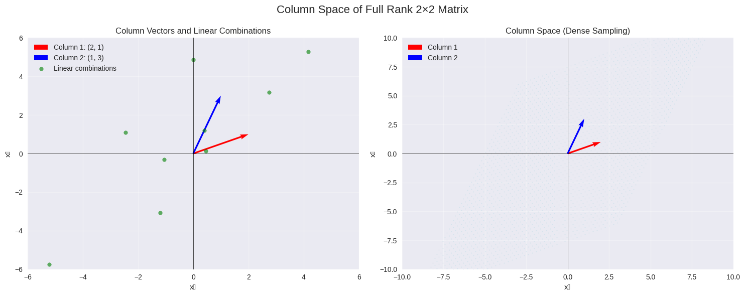
6.4.7.3. Visualizing the Column Space in 2D#

For a 2×2 matrix with full rank, the column space spans all of $\mathbb{R}^2$. Let’s visualize this:

Show code cell content

Hide code cell content

def plot_column_space_2d(A, title="Column Space Visualization"):
    """
    Visualize the column space of a 2x2 matrix
    """
    fig, (ax1, ax2) = plt.subplots(1, 2, figsize=(15, 6))

    # Plot 1: Column vectors and their span
    col1, col2 = A[:, 0], A[:, 1]

    # Plot column vectors
    ax1.quiver(
        0,
        0,
        col1[0],
        col1[1],
        angles="xy",
        scale_units="xy",
        scale=1,
        color="red",
        width=0.005,
        label=f"Column 1: ({col1[0]}, {col1[1]})",
    )
    ax1.quiver(
        0,
        0,
        col2[0],
        col2[1],
        angles="xy",
        scale_units="xy",
        scale=1,
        color="blue",
        width=0.005,
        label=f"Column 2: ({col2[0]}, {col2[1]})",
    )

    # Show some linear combinations
    coeffs = np.random.uniform(-2, 2, (10, 2))
    linear_combinations = A @ coeffs.T

    ax1.scatter(
        linear_combinations[0],
        linear_combinations[1],
        c="green",
        alpha=0.6,
        s=30,
        label="Linear combinations",
    )

    ax1.set_xlim(-6, 6)
    ax1.set_ylim(-6, 6)
    ax1.grid(True, alpha=0.3)
    ax1.axhline(y=0, color="k", linewidth=0.5)
    ax1.axvline(x=0, color="k", linewidth=0.5)
    ax1.set_xlabel("x₁")
    ax1.set_ylabel("x₂")
    ax1.legend()
    ax1.set_title("Column Vectors and Linear Combinations")

    # Plot 2: Dense sampling of the column space
    # Create a grid of coefficients
    c1_range = np.linspace(-3, 3, 50)
    c2_range = np.linspace(-3, 3, 50)
    C1, C2 = np.meshgrid(c1_range, c2_range)

    # Compute all linear combinations
    X = col1[0] * C1 + col2[0] * C2
    Y = col1[1] * C1 + col2[1] * C2

    ax2.scatter(X.flatten(), Y.flatten(), c="lightblue", alpha=0.3, s=1)
    ax2.quiver(
        0,
        0,
        col1[0],
        col1[1],
        angles="xy",
        scale_units="xy",
        scale=1,
        color="red",
        width=0.005,
        label="Column 1",
    )
    ax2.quiver(
        0,
        0,
        col2[0],
        col2[1],
        angles="xy",
        scale_units="xy",
        scale=1,
        color="blue",
        width=0.005,
        label="Column 2",
    )

    ax2.set_xlim(-10, 10)
    ax2.set_ylim(-10, 10)
    ax2.grid(True, alpha=0.3)
    ax2.axhline(y=0, color="k", linewidth=0.5)
    ax2.axvline(x=0, color="k", linewidth=0.5)
    ax2.set_xlabel("x₁")
    ax2.set_ylabel("x₂")
    ax2.legend()
    ax2.set_title("Column Space (Dense Sampling)")

    plt.suptitle(title, fontsize=16)
    plt.tight_layout()
    plt.show()

# Visualize the column space of our simple matrix
plot_column_space_2d(A_simple, "Column Space of Full Rank 2×2 Matrix")

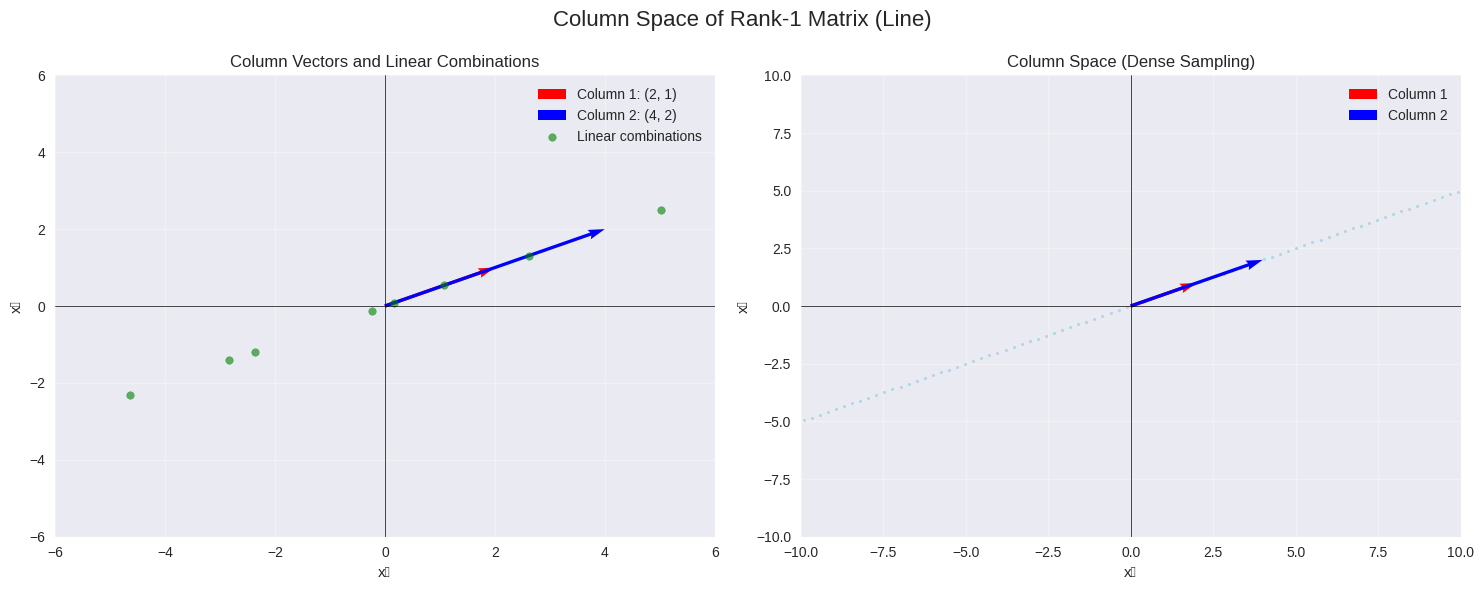
../_images/2a14902da030ebb07fe568479d78ea82b39429a8ff57a38d0f5cda3a733b4211.png

6.4.7.4. Column Space with Linearly Dependent Columns#

Now let’s look at a matrix where the columns are linearly dependent:

# Matrix with linearly dependent columns
A_dependent = np.array([[2, 4], [1, 2]])

print("Matrix A (linearly dependent columns):")
print(A_dependent)
print(f"Rank: {np.linalg.matrix_rank(A_dependent)}")

# Note: Column 2 is 2 * Column 1
print(f"\nColumn 1: {A_dependent[:, 0]}")
print(f"Column 2: {A_dependent[:, 1]}")
print(f"Column 2 / Column 1: {A_dependent[:, 1] / A_dependent[:, 0]}")

plot_column_space_2d(A_dependent, "Column Space of Rank-1 Matrix (Line)")

Matrix A (linearly dependent columns):
[[2 4]
 [1 2]]
Rank: 1

Column 1: [2 1]
Column 2: [4 2]
Column 2 / Column 1: [2. 2.]

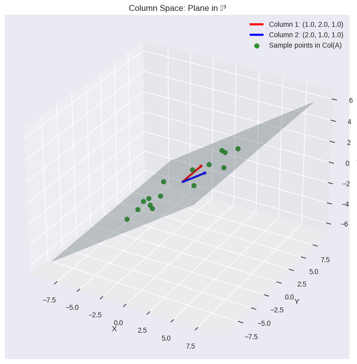
../_images/c93236b5280aa29d51a3fd5792041acc0f15012b5391f84a97198b9515df0aea.png

6.4.7.5. 3D Column Space Visualization#

Let’s explore the column space of a 3×2 matrix, which will be a plane in 3D space:

# Example 3x2 matrix
A_3d = np.array([[1, 2], [2, 1], [1, 1]])

print("3×2 Matrix A:")
print(A_3d)
print(f"Rank: {np.linalg.matrix_rank(A_3d)}")

plot_column_space_3d(A_3d, "Column Space: Plane in ℝ³")

3×2 Matrix A:
[[1 2]
 [2 1]
 [1 1]]
Rank: 2

../_images/6455e310b70110f46c514799762508490d29587380869ea9c580b38ab32d09cd.png

6.4.8. Understanding the Null Space#

6.4.8.1. Definition#

The null space (also called the kernel) of an $m \times n$ matrix $A$ is the set of all vectors $\mathbf{x}$ that satisfy $A\mathbf{x} = \mathbf{0}$. Mathematically:

\[\text{Null}(A) = \{\mathbf{x} \in \mathbb{R}^n : A\mathbf{x} = \mathbf{0}\}\]

6.4.8.2. Key Properties#

The null space is a subspace of $\mathbb{R}^n$
The dimension of the null space is called the nullity of the matrix
Rank-Nullity Theorem: For an $m \times n$ matrix $A$: $$\text{rank}(A) + \text{nullity}(A) = n$$

def analyze_null_space(A, name="Matrix A"):
    """
    Analyze and display null space properties
    """
    print(f"\n{name}:")
    print(A)
    print(f"Shape: {A.shape}")

    rank = np.linalg.matrix_rank(A)
    n = A.shape[1]
    nullity = n - rank

    print(f"Rank: {rank}")
    print(f"Nullity: {nullity}")
    print(f"Rank + Nullity = {rank + nullity} (should equal {n})")

    # Compute null space
    if nullity > 0:
        null_basis = null_space(A)
        print(f"\nNull space basis vectors:")
        for i, vec in enumerate(null_basis.T):
            print(f"  v{i+1} = {vec}")
            # Verify it's in the null space
            result = A @ vec
            print(f"  A·v{i+1} = {result} (should be ~0)")
    else:
        print("\nNull space contains only the zero vector.")

    return rank, nullity


# Example 1: Full rank matrix (null space = {0})
A1 = np.array([[1, 2], [3, 4]])
analyze_null_space(A1, "Full Rank 2×2 Matrix")

# Example 2: Matrix with non-trivial null space
A2 = np.array([[1, 2, 1], [2, 4, 2], [1, 2, 1]])
analyze_null_space(A2, "Rank-1 3×3 Matrix")

Full Rank 2×2 Matrix:
[[1 2]
 [3 4]]
Shape: (2, 2)
Rank: 2
Nullity: 0
Rank + Nullity = 2 (should equal 2)

Null space contains only the zero vector.

Rank-1 3×3 Matrix:
[[1 2 1]
 [2 4 2]
 [1 2 1]]
Shape: (3, 3)
Rank: 1
Nullity: 2
Rank + Nullity = 3 (should equal 3)

Null space basis vectors:
  v1 = [-0.91287093  0.36514837  0.18257419]
  A·v1 = [-4.99600361e-16 -9.99200722e-16 -4.99600361e-16] (should be ~0)
  v2 = [-0.          0.4472136  -0.89442719]
  A·v2 = [0. 0. 0.] (should be ~0)

(1, 2)

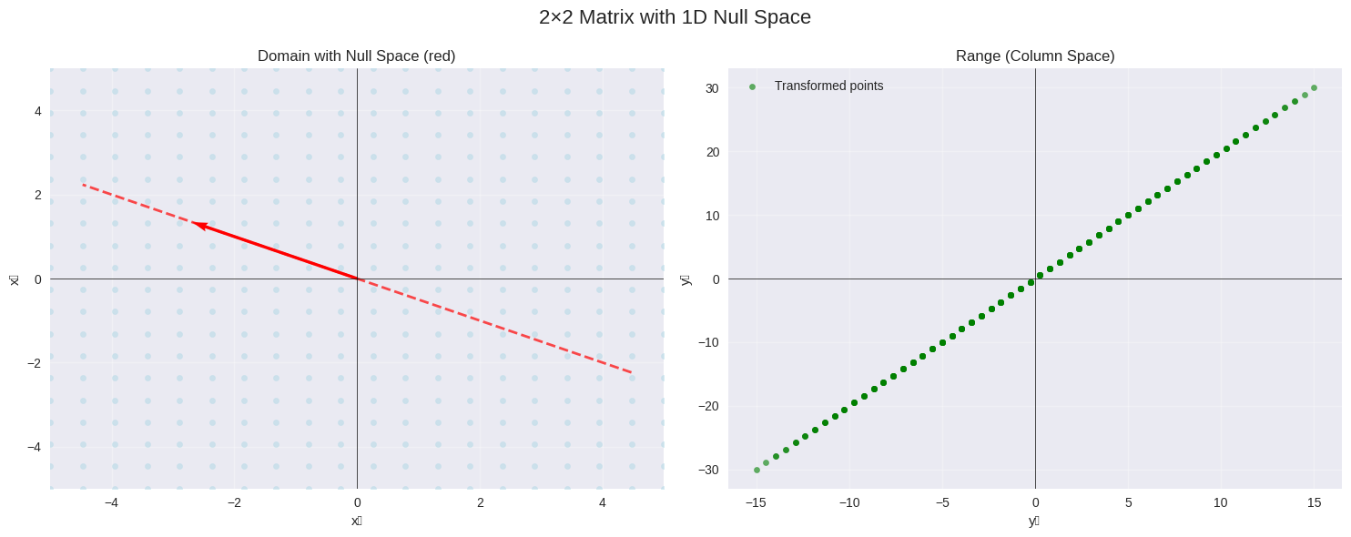
6.4.8.3. Visualizing the Null Space#

Let’s create visualizations for different types of null spaces:

Show code cell content

Hide code cell content

def plot_null_space_2d(A, title="Null Space Visualization"):
    """
    Visualize null space for matrices with 2D domain
    """
    if A.shape[1] != 2:
        print("This function is for matrices with 2 columns only.")
        return

    fig, (ax1, ax2) = plt.subplots(1, 2, figsize=(15, 6))

    # Create a grid of points
    x = np.linspace(-5, 5, 20)
    y = np.linspace(-5, 5, 20)
    X, Y = np.meshgrid(x, y)

    # Flatten for easier computation
    points = np.vstack([X.flatten(), Y.flatten()])

    # Transform points through matrix A
    transformed = A @ points

    # Plot 1: Original domain with null space highlighted
    ax1.scatter(
        points[0], points[1], c="lightblue", alpha=0.5, s=20, label="Domain points"
    )

    # Find and highlight null space
    null_basis = null_space(A)
    nullity = null_basis.shape[1]

    if nullity > 0:
        # Plot null space basis vectors
        for i, vec in enumerate(null_basis.T):
            # Scale for visibility
            scale_factor = 3
            ax1.quiver(
                0,
                0,
                vec[0] * scale_factor,
                vec[1] * scale_factor,
                angles="xy",
                scale_units="xy",
                scale=1,
                color="red",
                width=0.005,
                label=f"Null space basis {i+1}",
            )

            # Plot the null space line/plane
            t = np.linspace(-5, 5, 100)
            null_line = np.outer(vec, t)
            ax1.plot(null_line[0], null_line[1], "r--", alpha=0.7, linewidth=2)

        ax1.set_title("Domain with Null Space (red)")
    else:
        ax1.plot(0, 0, "ro", markersize=8, label="Null space (only origin)")
        ax1.set_title("Domain (null space = {0})")

    ax1.set_xlim(-5, 5)
    ax1.set_ylim(-5, 5)
    ax1.grid(True, alpha=0.3)
    ax1.axhline(y=0, color="k", linewidth=0.5)
    ax1.axvline(x=0, color="k", linewidth=0.5)
    ax1.set_xlabel("x₁")
    ax1.set_ylabel("x₂")
    # ax1.legend()

    # Plot 2: Range (column space)
    if A.shape[0] == 2:
        ax2.scatter(
            transformed[0],
            transformed[1],
            c="green",
            alpha=0.6,
            s=20,
            label="Transformed points",
        )
        ax2.set_xlabel("y₁")
        ax2.set_ylabel("y₂")
    else:
        # For higher dimensional output, just show first two components
        ax2.scatter(
            transformed[0],
            transformed[1],
            c="green",
            alpha=0.6,
            s=20,
            label="First 2 components",
        )
        ax2.set_xlabel("y₁")
        ax2.set_ylabel("y₂")

    ax2.set_title("Range (Column Space)")
    ax2.grid(True, alpha=0.3)
    ax2.axhline(y=0, color="k", linewidth=0.5)
    ax2.axvline(x=0, color="k", linewidth=0.5)
    ax2.legend()

    plt.suptitle(title, fontsize=16)
    plt.tight_layout()
    plt.show()

# Example with non-trivial null space
A_null_example = np.array([[1, 2], [2, 4]])

print("Matrix with 1D null space:")
analyze_null_space(A_null_example)
plot_null_space_2d(A_null_example, "2×2 Matrix with 1D Null Space")

Matrix with 1D null space:

Matrix A:
[[1 2]
 [2 4]]
Shape: (2, 2)
Rank: 1
Nullity: 1
Rank + Nullity = 2 (should equal 2)

Null space basis vectors:
  v1 = [-0.89442719  0.4472136 ]
  A·v1 = [0. 0.] (should be ~0)

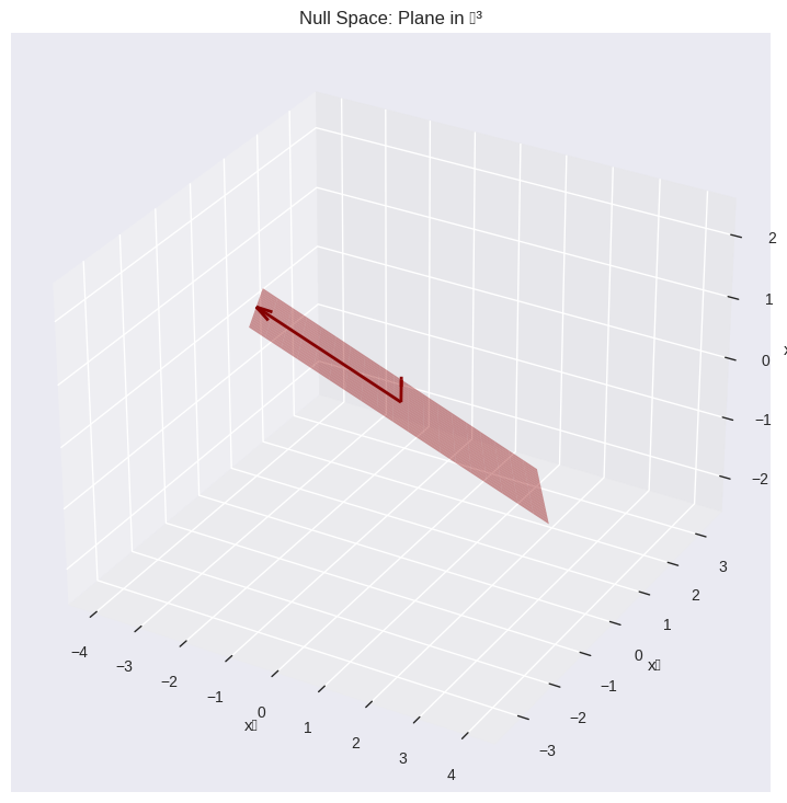
../_images/9d988000363e6fb777a4eb546c2bf2b24a28d194912dffc3aed579109848d313.png

6.4.8.4. 3D Null Space Example#

Let’s look at a 3×3 matrix with a 2D null space:

Show code cell content

Hide code cell content

def plot_null_space_3d(A, title="3D Null Space Visualization"):
    """
    Visualize null space in 3D
    """
    if A.shape[1] != 3:
        print("This function is for 3-column matrices only.")
        return

    fig = plt.figure(figsize=(12, 9))
    ax = fig.add_subplot(111, projection="3d")

    # Get null space basis
    null_basis = null_space(A)
    nullity = null_basis.shape[1]

    if nullity == 0:
        ax.scatter([0], [0], [0], c="red", s=100, label="Null space (origin only)")
    elif nullity == 1:
        # 1D null space (line through origin)
        vec = null_basis[:, 0]
        t = np.linspace(-5, 5, 100)
        line = np.outer(vec, t)
        ax.plot(line[0], line[1], line[2], "r-", linewidth=3, label="Null space (line)")
        ax.quiver(
            0,
            0,
            0,
            vec[0] * 3,
            vec[1] * 3,
            vec[2] * 3,
            color="red",
            arrow_length_ratio=0.1,
            linewidth=2,
        )
    elif nullity == 2:
        # 2D null space (plane through origin)
        vec1, vec2 = null_basis[:, 0], null_basis[:, 1]

        # Create plane
        t1 = np.linspace(-3, 3, 20)
        t2 = np.linspace(-3, 3, 20)
        T1, T2 = np.meshgrid(t1, t2)

        X = vec1[0] * T1 + vec2[0] * T2
        Y = vec1[1] * T1 + vec2[1] * T2
        Z = vec1[2] * T1 + vec2[2] * T2

        ax.plot_surface(X, Y, Z, alpha=0.4, color="red", label="Null space (plane)")

        # Plot basis vectors
        ax.quiver(
            0,
            0,
            0,
            vec1[0] * 3,
            vec1[1] * 3,
            vec1[2] * 3,
            color="darkred",
            arrow_length_ratio=0.1,
            linewidth=2,
            label="Basis 1",
        )
        ax.quiver(
            0,
            0,
            0,
            vec2[0] * 3,
            vec2[1] * 3,
            vec2[2] * 3,
            color="maroon",
            arrow_length_ratio=0.1,
            linewidth=2,
            label="Basis 2",
        )

    ax.set_xlabel("x₁")
    ax.set_ylabel("x₂")
    ax.set_zlabel("x₃")
    ax.set_title(title)
    # ax.legend()

    plt.show()

# Example: 1×3 matrix (2D null space)
A_2d_null = np.array([[1, 2, 3]])

print("1×3 Matrix (2D null space):")
analyze_null_space(A_2d_null)
plot_null_space_3d(A_2d_null, "Null Space: Plane in ℝ³")

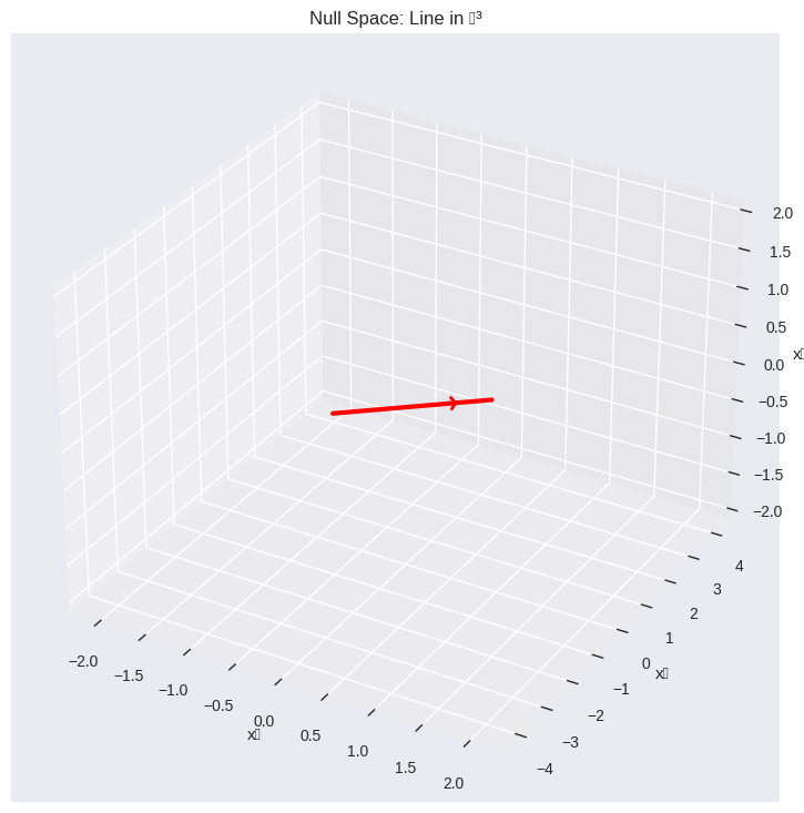
# Example: 2×3 matrix (1D null space)
A_1d_null = np.array([[1, 2, 3], [4, 5, 6]])

print("\n2×3 Matrix (1D null space):")
analyze_null_space(A_1d_null)
plot_null_space_3d(A_1d_null, "Null Space: Line in ℝ³")

1×3 Matrix (2D null space):

Matrix A:
[[1 2 3]]
Shape: (1, 3)
Rank: 1
Nullity: 2
Rank + Nullity = 3 (should equal 3)

Null space basis vectors:
  v1 = [-0.53452248  0.77454192 -0.33818712]
  A·v1 = [-5.55111512e-17] (should be ~0)
  v2 = [-0.80178373 -0.33818712  0.49271932]
  A·v2 = [-6.66133815e-16] (should be ~0)

../_images/897ae8a5a885d76e1fe0d594020d39beed83de504bdd2f14f917426853b907ba.png

2×3 Matrix (1D null space):

Matrix A:
[[1 2 3]
 [4 5 6]]
Shape: (2, 3)
Rank: 2
Nullity: 1
Rank + Nullity = 3 (should equal 3)

Null space basis vectors:
  v1 = [ 0.40824829 -0.81649658  0.40824829]
  A·v1 = [ 1.66533454e-16 -5.55111512e-16] (should be ~0)

../_images/6bee2745f635445c1290e69fb68cd7f0586eb0f85756fe0859f4055f30c3474b.png

6.4.9. The Fundamental Relationship: Column Space ⊥ Left Null Space#

There’s a beautiful orthogonality relationship between the four fundamental subspaces of a matrix:

For an $m \times n$ matrix $A$:

Column Space: $\text{Col}(A) \subset \mathbb{R}^m$
Left Null Space: $\text{Null}(A^T) \subset \mathbb{R}^m$
Row Space: $\text{Col}(A^T) \subset \mathbb{R}^n$
Null Space: $\text{Null}(A) \subset \mathbb{R}^n$

Key Orthogonality Relations:

$\text{Col}(A) \perp \text{Null}(A^T)$
$\text{Col}(A^T) \perp \text{Null}(A)$

def analyze_four_subspaces(A):
    """
    Analyze all four fundamental subspaces of a matrix
    """
    m, n = A.shape

    print(f"Matrix A ({m}×{n}):")
    print(A)
    print(f"\nRank: {np.linalg.matrix_rank(A)}")

    # Column space
    col_rank = np.linalg.matrix_rank(A)
    print(f"\n1. Column Space (in ℝ^{m}):")
    print(f"   Dimension: {col_rank}")

    # Row space
    row_rank = np.linalg.matrix_rank(A.T)
    print(f"\n2. Row Space (in ℝ^{n}):")
    print(f"   Dimension: {row_rank}")

    # Null space
    null_A = null_space(A)
    nullity_A = null_A.shape[1]
    print(f"\n3. Null Space (in ℝ^{n}):")
    print(f"   Dimension: {nullity_A}")
    if nullity_A > 0:
        print(f"   Basis vectors:")
        for i, vec in enumerate(null_A.T):
            print(f"   v{i+1} = {vec}")

    # Left null space
    left_null_A = null_space(A.T)
    left_nullity_A = left_null_A.shape[1]
    print(f"\n4. Left Null Space (in ℝ^{m}):")
    print(f"   Dimension: {left_nullity_A}")
    if left_nullity_A > 0:
        print(f"   Basis vectors:")
        for i, vec in enumerate(left_null_A.T):
            print(f"   w{i+1} = {vec}")

    # Verify rank-nullity theorem
    print(f"\nRank-Nullity Verification:")
    print(
        f"   rank(A) + nullity(A) = {col_rank} + {nullity_A} = {col_rank + nullity_A} (should = {n})"
    )
    print(
        f"   rank(A^T) + nullity(A^T) = {row_rank} + {left_nullity_A} = {row_rank + left_nullity_A} (should = {m})"
    )

    # Test orthogonality
    print(f"\nOrthogonality Tests:")
    if nullity_A > 0 and A.shape[1] <= 3:  # Only for small examples
        # Test if null space is orthogonal to row space
        for i, null_vec in enumerate(null_A.T):
            for j in range(min(A.shape[0], 3)):  # Test first few rows
                dot_product = np.dot(A[j], null_vec)
                print(
                    f"   Row {j+1} · null_vec_{i+1} = {dot_product:.6f} (should be ≈ 0)"
                )


# Example matrix
A_example = np.array([[1, 2, 3], [4, 5, 6], [7, 8, 9]])

analyze_four_subspaces(A_example)

Matrix A (3×3):
[[1 2 3]
 [4 5 6]
 [7 8 9]]

Rank: 2

1. Column Space (in ℝ^3):
   Dimension: 2

2. Row Space (in ℝ^3):
   Dimension: 2

3. Null Space (in ℝ^3):
   Dimension: 1
   Basis vectors:
   v1 = [-0.40824829  0.81649658 -0.40824829]

4. Left Null Space (in ℝ^3):
   Dimension: 1
   Basis vectors:
   w1 = [ 0.40824829 -0.81649658  0.40824829]

Rank-Nullity Verification:
   rank(A) + nullity(A) = 2 + 1 = 3 (should = 3)
   rank(A^T) + nullity(A^T) = 2 + 1 = 3 (should = 3)

Orthogonality Tests:
   Row 1 · null_vec_1 = -0.000000 (should be ≈ 0)
   Row 2 · null_vec_1 = 0.000000 (should be ≈ 0)
   Row 3 · null_vec_1 = 0.000000 (should be ≈ 0)

6.4.10. Interactive Exploration#

Let’s create an interactive tool to explore how changing matrix entries affects the column space and null space:

def explore_matrix_spaces(a11=1, a12=2, a21=3, a22=4):
    """
    Interactive exploration of 2x2 matrix spaces
    """
    A = np.array([[a11, a12], [a21, a22]])

    print(f"Matrix A:")
    print(A)

    det_A = np.linalg.det(A)
    rank_A = np.linalg.matrix_rank(A)

    print(f"\nDeterminant: {det_A:.4f}")
    print(f"Rank: {rank_A}")

    if abs(det_A) < 1e-10:
        print("Matrix is singular (not invertible)")
        print("Column space is a line (1D)")
        print("Null space is a line (1D)")
    else:
        print("Matrix is non-singular (invertible)")
        print("Column space is all of ℝ² (2D)")
        print("Null space is just {0} (0D)")

    # Visualize
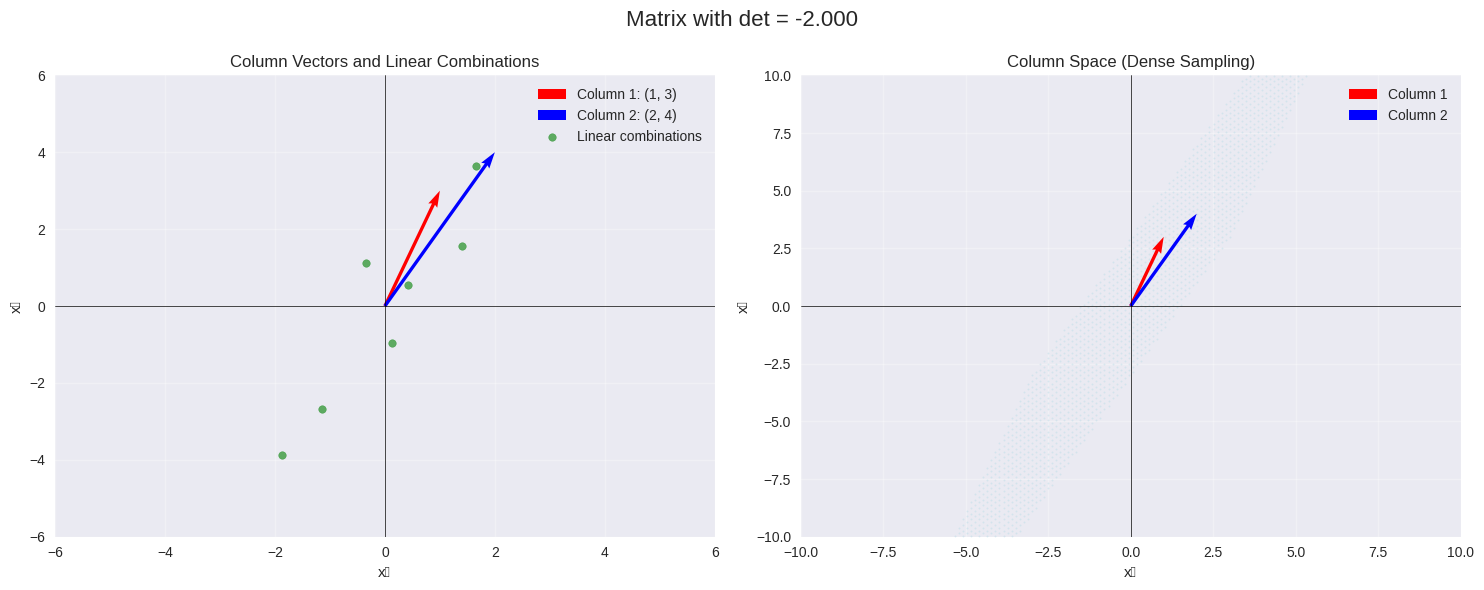
    plot_column_space_2d(A, f"Matrix with det = {det_A:.3f}")
    if rank_A < 2:
        plot_null_space_2d(A, f"Null Space (rank = {rank_A})")


# Try different matrices
print("Example 1: Non-singular matrix")
explore_matrix_spaces(1, 2, 3, 4)

print("\n" + "=" * 50)
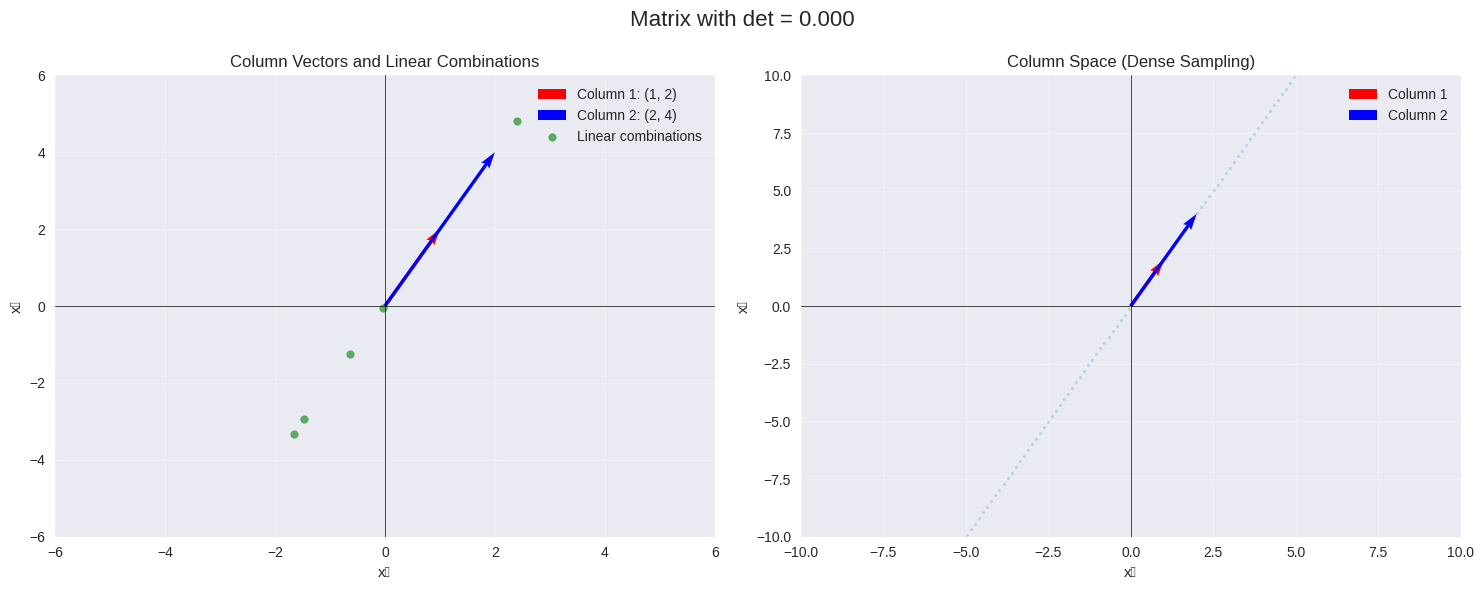
print("Example 2: Singular matrix")
explore_matrix_spaces(1, 2, 2, 4)

Example 1: Non-singular matrix
Matrix A:
[[1 2]
 [3 4]]

Determinant: -2.0000
Rank: 2
Matrix is non-singular (invertible)
Column space is all of ℝ² (2D)
Null space is just {0} (0D)

../_images/042cec55af3847b34a8672cec4fc756edaf5849430556021f7d5720dad6b2329.png

==================================================
Example 2: Singular matrix
Matrix A:
[[1 2]
 [2 4]]

Determinant: 0.0000
Rank: 1
Matrix is singular (not invertible)
Column space is a line (1D)
Null space is a line (1D)

../_images/19c5e1724ab523ac9ac4c4d30d6972beb7b4d23e806e0b3c359cfaec64ec6686.png

../_images/489eef05581361fc32460e6e606d50abdf473b3dcc28dd74595bda725375df35.png

6.4.11. Practical Applications#

6.4.11.1. Application 1: Solving Linear Systems#

Understanding column space and null space helps us analyze the solvability of linear systems $A\mathbf{x} = \mathbf{b}$:

def analyze_linear_system(A, b):
    """
    Analyze the solvability of Ax = b
    """
    print("Linear System Analysis: Ax = b")
    print(f"\nMatrix A:")
    print(A)
    print(f"\nVector b: {b}")

    # Check if b is in the column space of A
    augmented = np.column_stack([A, b])
    rank_A = np.linalg.matrix_rank(A)
    rank_augmented = np.linalg.matrix_rank(augmented)

    print(f"\nRank of A: {rank_A}")
    print(f"Rank of [A|b]: {rank_augmented}")

    if rank_A == rank_augmented:
        print("\n✓ System is CONSISTENT (b is in the column space of A)")

        # Check for uniqueness
        n = A.shape[1]
        if rank_A == n:
            print("✓ Solution is UNIQUE (null space is trivial)")
            try:
                x = np.linalg.solve(A, b)
                print(f"Solution: x = {x}")
                print(f"Verification: Ax = {A @ x}")
            except:
                x = np.linalg.lstsq(A, b, rcond=None)[0]
                print(f"Least squares solution: x = {x}")
        else:
            print(
                f"✓ INFINITELY MANY solutions (null space has dimension {n - rank_A})"
            )
            x_particular = np.linalg.lstsq(A, b, rcond=None)[0]
            print(f"Particular solution: x_p = {x_particular}")

            null_basis = null_space(A)
            print(f"General solution: x = x_p + c₁v₁ + c₂v₂ + ... where:")
            for i, vec in enumerate(null_basis.T):
                print(f"  v{i+1} = {vec}")
    else:
        print("\n✗ System is INCONSISTENT (b is not in the column space of A)")
        print("No exact solution exists.")

        # Compute least squares solution
        x_ls = np.linalg.lstsq(A, b, rcond=None)[0]
        residual = A @ x_ls - b
        print(f"\nLeast squares solution: x = {x_ls}")
        print(f"Residual: ||Ax - b|| = {np.linalg.norm(residual):.6f}")


# Example 1: Unique solution
A1 = np.array([[1, 2], [3, 4]])
b1 = np.array([5, 6])
analyze_linear_system(A1, b1)

print("\n" + "=" * 60)

# Example 2: Infinitely many solutions
A2 = np.array([[1, 2, 3], [4, 5, 6]])
b2 = np.array([1, 2])
analyze_linear_system(A2, b2)

print("\n" + "=" * 60)

# Example 3: No solution
A3 = np.array([[1, 2], [2, 4]])
b3 = np.array([1, 3])
analyze_linear_system(A3, b3)

Linear System Analysis: Ax = b

Matrix A:
[[1 2]
 [3 4]]

Vector b: [5 6]

Rank of A: 2
Rank of [A|b]: 2

✓ System is CONSISTENT (b is in the column space of A)
✓ Solution is UNIQUE (null space is trivial)
Solution: x = [-4.   4.5]
Verification: Ax = [5. 6.]

============================================================
Linear System Analysis: Ax = b

Matrix A:
[[1 2 3]
 [4 5 6]]

Vector b: [1 2]

Rank of A: 2
Rank of [A|b]: 2

✓ System is CONSISTENT (b is in the column space of A)
✓ INFINITELY MANY solutions (null space has dimension 1)
Particular solution: x_p = [-0.05555556  0.11111111  0.27777778]
General solution: x = x_p + c₁v₁ + c₂v₂ + ... where:
  v1 = [ 0.40824829 -0.81649658  0.40824829]

============================================================
Linear System Analysis: Ax = b

Matrix A:
[[1 2]
 [2 4]]

Vector b: [1 3]

Rank of A: 1
Rank of [A|b]: 2

✗ System is INCONSISTENT (b is not in the column space of A)
No exact solution exists.

Least squares solution: x = [0.28 0.56]
Residual: ||Ax - b|| = 0.447214

6.4.11.2. Application 2: Principal Component Analysis (PCA)#

The column space concept is fundamental to understanding dimensionality reduction techniques like PCA:

def demonstrate_pca_column_space():
    """
    Show how PCA relates to column space
    """
    # Generate sample data
    np.random.seed(42)
    n_samples = 100

    # Create correlated 2D data
    X_original = np.random.randn(n_samples, 2)
    # Make second dimension correlated with first
    X_original[:, 1] = 0.5 * X_original[:, 0] + 0.3 * X_original[:, 1]

    # Center the data
    X = X_original - np.mean(X_original, axis=0)

    # Compute SVD
    U, s, Vt = np.linalg.svd(X, full_matrices=False)

    print("PCA Analysis using SVD")
    print(f"Data shape: {X.shape}")
    print(f"Singular values: {s}")
    print(f"Explained variance ratio: {s**2 / np.sum(s**2)}")

    # Principal components (columns of V)
    V = Vt.T
    print(f"\nPrincipal components (columns of V):")
    print(f"PC1: {V[:, 0]}")
    print(f"PC2: {V[:, 1]}")

    # Project onto first principal component
    X_projected_1d = X @ V[:, 0:1] @ V[:, 0:1].T

    # Create visualization
    fig, ((ax1, ax2), (ax3, ax4)) = plt.subplots(2, 2, figsize=(15, 12))

    # Plot 1: Original data with principal directions
    ax1.scatter(X[:, 0], X[:, 1], alpha=0.6, c="blue", label="Original data")

    # Plot principal component directions
    scale = 3
    ax1.arrow(
        0,
        0,
        V[0, 0] * scale,
        V[1, 0] * scale,
        head_width=0.1,
        head_length=0.1,
        fc="red",
        ec="red",
        label=f"PC1 (σ={s[0]:.2f})",
    )
    ax1.arrow(
        0,
        0,
        V[0, 1] * scale,
        V[1, 1] * scale,
        head_width=0.1,
        head_length=0.1,
        fc="green",
        ec="green",
        label=f"PC2 (σ={s[1]:.2f})",
    )

    ax1.set_xlabel("X₁")
    ax1.set_ylabel("X₂")
    ax1.set_title("Original Data with Principal Components")
    ax1.grid(True, alpha=0.3)
    ax1.legend()
    ax1.axis("equal")

    # Plot 2: Data in PC coordinate system
    X_pc = X @ V  # Transform to PC coordinates
    ax2.scatter(X_pc[:, 0], X_pc[:, 1], alpha=0.6, c="blue")
    ax2.set_xlabel("PC1")
    ax2.set_ylabel("PC2")
    ax2.set_title("Data in Principal Component Coordinates")
    ax2.grid(True, alpha=0.3)
    ax2.axis("equal")

    # Plot 3: 1D projection (column space of first PC)
    ax3.scatter(X[:, 0], X[:, 1], alpha=0.3, c="lightblue", label="Original data")
    ax3.scatter(
        X_projected_1d[:, 0],
        X_projected_1d[:, 1],
        alpha=0.8,
        c="red",
        s=20,
        label="Projection onto PC1",
    )

    # Show the 1D subspace (line through origin)
    t = np.linspace(-4, 4, 100)
    pc1_line = np.outer(V[:, 0], t)
    ax3.plot(
        pc1_line[0], pc1_line[1], "r--", alpha=0.7, linewidth=2, label="PC1 subspace"
    )

    ax3.set_xlabel("X₁")
    ax3.set_ylabel("X₂")
    ax3.set_title("Projection onto 1D Column Space (PC1)")
    ax3.grid(True, alpha=0.3)
    ax3.legend()
    ax3.axis("equal")

    # Plot 4: Explained variance
    variance_explained = s**2 / np.sum(s**2)
    cumsum_var = np.cumsum(variance_explained)

    ax4.bar(range(1, len(s) + 1), variance_explained, alpha=0.7, label="Individual")
    ax4.plot(range(1, len(s) + 1), cumsum_var, "ro-", label="Cumulative")
    ax4.set_xlabel("Principal Component")
    ax4.set_ylabel("Explained Variance Ratio")
    ax4.set_title("Explained Variance by Principal Components")
    ax4.legend()
    ax4.grid(True, alpha=0.3)

    plt.tight_layout()
    plt.show()

    print(f"\nDimensionality Reduction Summary:")
    print(f"- Original data: 2D")
    print(f"- First PC captures {variance_explained[0]:.3f} of total variance")
    print(f"- Projection error (using 1D): {np.linalg.norm(X - X_projected_1d)**2:.3f}")
    print(f"- The 1D column space spanned by PC1 contains most information!")


demonstrate_pca_column_space()

PCA Analysis using SVD
Data shape: (100, 2)
Singular values: [9.67280091 2.62490665]
Explained variance ratio: [0.93140951 0.06859049]

Principal components (columns of V):
PC1: [-0.87066995 -0.49186771]
PC2: [ 0.49186771 -0.87066995]

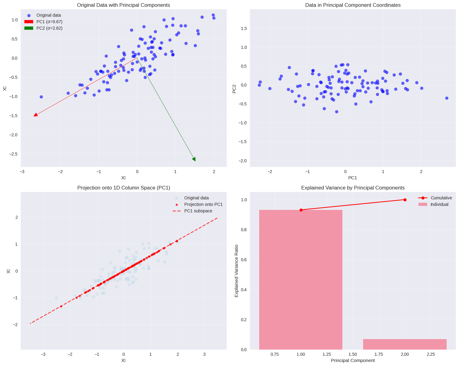
../_images/5887101b9317ac9769bb957e6875c6277360b9c00cb27b00c39f4ce8aacda05e.png

Dimensionality Reduction Summary:
- Original data: 2D
- First PC captures 0.931 of total variance
- Projection error (using 1D): 6.890
- The 1D column space spanned by PC1 contains most information!

6.4.12. Summary and Key Takeaways#

6.4.12.1. Matrix Rank#

Definition: Maximum number of linearly independent columns (or rows)
Geometric interpretation: “Effective dimensionality” of the transformation
Range: $0 \leq \text{rank}(A) \leq \min(m,n)$
Applications: Determines solvability, invertibility, and dimensional reduction

6.4.12.2. Inverse Matrices#

Definition: Matrix $A^{-1}$ such that $AA^{-1} = A^{-1}A = I$
Geometric interpretation: “Undoes” the transformation of $A$
Existence: Only for square, full-rank matrices (det ≠ 0)
Applications: Solving systems uniquely, reversing transformations

6.4.12.3. Column Space#

Definition: All possible linear combinations of the columns of matrix $A$
Geometric interpretation: The “span” of the column vectors
Dimension: Equals the rank of the matrix
Applications: Determines which vectors $\mathbf{b}$ make $A\mathbf{x} = \mathbf{b}$ solvable

6.4.12.4. Null Space#

Definition: All vectors $\mathbf{x}$ such that $A\mathbf{x} = \mathbf{0}$
Geometric interpretation: The “kernel” of the linear transformation
Dimension: Called the nullity, equals $n - \text{rank}(A)$
Applications: Describes the “freedom” in solutions to $A\mathbf{x} = \mathbf{b}$

6.4.12.5. 🔗 Fundamental Connections#

Rank-Nullity Theorem: $\text{rank}(A) + \text{nullity}(A) = n$
Invertibility: $A^{-1}$ exists ⟺ full rank ⟺ det ≠ 0 ⟺ trivial null space
Orthogonality: Column space ⊥ Left null space
Four Fundamental Subspaces: Column, row, null, and left null spaces
Decision Chain:
- Full rank → Invertible → Unique solutions → Trivial null space
- Rank deficient → Not invertible → Multiple/no solutions → Non-trivial null space

6.4.12.6. 🎯 Practical Applications#

Linear systems: Understanding existence and uniqueness of solutions
Data analysis: PCA, dimensionality reduction, feature extraction
Machine learning: Model capacity, overfitting, regularization
Engineering: Control systems, signal processing, optimization
Computer graphics: Transformations, projections, rotations

6.4.12.7. 🎬 Recommended Viewing#

Don’t miss the excellent 3Blue1Brown video that inspired this notebook: “Inverse matrices, column space and null space” - https://www.youtube.com/watch?v=uQhTuRlWMxw

# Final interactive exploration
print("🎯 Final Challenge: Explore Your Own Matrix!")
print("\nTry modifying this matrix and observe how the spaces change:")

# You can modify these values
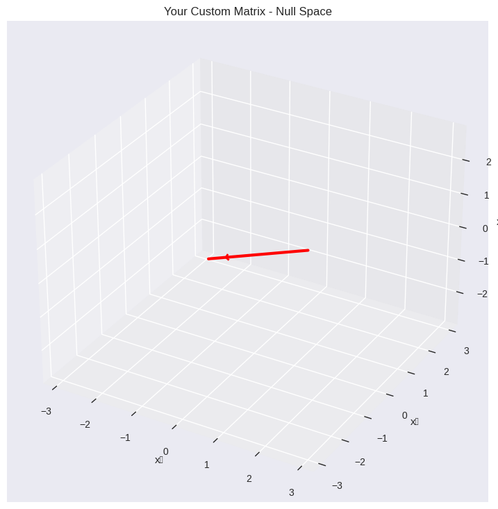
custom_matrix = np.array([[1, 2, 1], [0, 1, 1], [1, 3, 2]])

print("\nYour custom matrix:")
analyze_four_subspaces(custom_matrix)

if custom_matrix.shape[1] == 3:
    plot_null_space_3d(custom_matrix, "Your Custom Matrix - Null Space")

print("\n" + "=" * 60)
print("🔬 Experiment Ideas:")
print("1. Change one entry and see how rank changes")
print("2. Make two rows identical - what happens to null space?")
print("3. Try a matrix where all rows sum to zero")
print("4. Create a matrix with rank 1 - visualize its column space")
print("5. Test different 2×2 matrices for invertibility")
print("6. See how determinant relates to rank and null space")
print("7. Create a rotation matrix and find its inverse")
print("8. Build a matrix where rank + nullity = n")
print("\n🎓 Remember: rank, inverse, column space, and null space are all connected!")
print("🎬 Watch: https://www.youtube.com/watch?v=uQhTuRlWMxw")
print("\nHappy exploring! 🚀")

🎯 Final Challenge: Explore Your Own Matrix!

Try modifying this matrix and observe how the spaces change:

Your custom matrix:
Matrix A (3×3):
[[1 2 1]
 [0 1 1]
 [1 3 2]]

Rank: 2

1. Column Space (in ℝ^3):
   Dimension: 2

2. Row Space (in ℝ^3):
   Dimension: 2

3. Null Space (in ℝ^3):
   Dimension: 1
   Basis vectors:
   v1 = [-0.57735027  0.57735027 -0.57735027]

4. Left Null Space (in ℝ^3):
   Dimension: 1
   Basis vectors:
   w1 = [-0.57735027 -0.57735027  0.57735027]

Rank-Nullity Verification:
   rank(A) + nullity(A) = 2 + 1 = 3 (should = 3)
   rank(A^T) + nullity(A^T) = 2 + 1 = 3 (should = 3)

Orthogonality Tests:
   Row 1 · null_vec_1 = 0.000000 (should be ≈ 0)
   Row 2 · null_vec_1 = 0.000000 (should be ≈ 0)
   Row 3 · null_vec_1 = 0.000000 (should be ≈ 0)

../_images/c0ee3504e51374325b4556b6b4ca3f914a480a361670d0b0a8a32579eda39ddd.png

============================================================
🔬 Experiment Ideas:
1. Change one entry and see how rank changes
2. Make two rows identical - what happens to null space?
3. Try a matrix where all rows sum to zero
4. Create a matrix with rank 1 - visualize its column space
5. Test different 2×2 matrices for invertibility
6. See how determinant relates to rank and null space
7. Create a rotation matrix and find its inverse
8. Build a matrix where rank + nullity = n

🎓 Remember: rank, inverse, column space, and null space are all connected!
🎬 Watch: https://www.youtube.com/watch?v=uQhTuRlWMxw

Happy exploring! 🚀

Column Space and Null Space

Contents

6.4. Column Space and Null Space#

6.4.1. Learning Objectives#

6.4.2. Prerequisites#

6.4.3. Reference Material#

6.4.4. Matrix Rank: The Foundation Concept#

6.4.4.1. Definition#

6.4.4.2. Key Properties#

6.4.4.3. Geometric Interpretation#

6.4.5. Inverse Matrices: Undoing Transformations#

6.4.5.1. Definition#

6.4.5.2. Key Properties#

6.4.5.3. When Does an Inverse NOT Exist?#

6.4.5.4. Geometric Interpretation#

6.4.6. The Big Picture: How Everything Connects#

6.4.6.1. 🔗 Fundamental Connections#

6.4.6.2. 🎯 Decision Tree#

6.4.7. Understanding the Column Space#

6.4.7.1. Definition#

6.4.7.2. Key Properties#

6.4.7.3. Visualizing the Column Space in 2D#

6.4.7.4. Column Space with Linearly Dependent Columns#

6.4.7.5. 3D Column Space Visualization#

6.4.8. Understanding the Null Space#

6.4.8.1. Definition#

6.4.8.2. Key Properties#

6.4.8.3. Visualizing the Null Space#

6.4.8.4. 3D Null Space Example#

6.4.9. The Fundamental Relationship: Column Space ⊥ Left Null Space#

6.4.10. Interactive Exploration#

6.4.11. Practical Applications#

6.4.11.1. Application 1: Solving Linear Systems#

6.4.11.2. Application 2: Principal Component Analysis (PCA)#

6.4.12. Summary and Key Takeaways#

6.4.12.1. Matrix Rank#

6.4.12.2. Inverse Matrices#

6.4.12.3. Column Space#

6.4.12.4. Null Space#

6.4.12.5. 🔗 Fundamental Connections#

6.4.12.6. 🎯 Practical Applications#

6.4.12.7. 🎬 Recommended Viewing#