6.5. Transforming coordinates

There are several transformations that can be performed on coordinates, such as translation, rotation, shearing, and reflection/mirroring. We are now going to address two simple ones: translation and rotation.

6.5.1. Translation

Translation means moving a vector or point \(x\) to the right and \(y\) up. A vector can be used to describe a translation. A translation by vector \((x,y)\) in 2D means that all points are moved \(x\) to the right and \(y\) up. To perform a translation, the vector is simply added to all points. For example, if you want to move a given point \((2,3)\) by \((1,2)\), you simply calculate \((2 + 1, 3 + 2) = (3, 5)\). So, the operation we perform here is addition.

6.5.2. Rotation

We have seen that a point in two dimensions can be written down as (x,y). A point can be rotated around the origin be multiplying it with a rotation matrix. We use the capital letter \(R\) to indicate such a matrix. The matrix has a parameter \(phi\) that is the angle to rotate counter clock-wise.

\[\begin{split} \begin{aligned} R(\phi) = \begin{bmatrix} \cos(\phi) & -\sin(\phi) \\ \sin(\phi) & \cos(\phi) \end{bmatrix}, \end{aligned} \end{split}\]

This reads as \(R\) is a rotation matrix that rotates anti-clockwise by angle \(\phi\). If you want to apply this to a point \((x,y)\), you can multiply the matrix with the vector.

\[\begin{split} \begin{aligned} \begin{bmatrix} \cos(\phi) & -\sin(\phi) \\ \sin(\phi) & \cos(\phi) \end{bmatrix} \times \begin{bmatrix} x \\ y \end{bmatrix} = \begin{bmatrix} x' \\ y' \end{bmatrix} \end{aligned} \end{split}\]

This read as multiplying the rotation matrix \(R\) with the vector \((x,y)\) will give you a new vector \((x', y')\) that is the result of rotating the original \((x,y)\) for angle \(\phi\). So, the operation here is multiplication.

6.6. Homogeneous coordinates

There is a mathematical trick by which all transformation, including translations, can be expressed as a matrix and performing the transformation is simply multiplying by that matrix. Do be able to do this, we must express coordinates as homogeneous coordinates. In homogenous coordinates one extra dimension is added to the original data. For example, if we have a 2D coordinate \((x,y)\), we can make the homogeneous coordinate by adding a 1 \((x, y, 1)\). To go back from homogeneous coordinates to ‘normal’ ones, we divide all components by the last value. For given example, it simply becomes \((x/1, y/1) = (x, y)\). So, if the last value is a one, we can simply remove that one and we have ‘ normal’ coordinates again. Below, we demonstrate this for 2D coordinates, but it can also be done for higher dimensions, such as 3D coordinates.

A translation of vector \((x,y)\) over \((t_{x}, t_{y})\) can now be written as a matrix, by putting the translation as the last column and all ones on the diagonal.

\[\begin{split} \begin{aligned} \begin{bmatrix} 1 & 0 & t_{x} \\ 0 & 1 & t_{y} \\ 0 & 0 & 1 \end{bmatrix} \times \begin{bmatrix} x \\ y \\ 1 \end{bmatrix} \end{aligned} \end{split}\]

Moreover, the rotation can be expressed by putting the rotation matrix \(R(\phi)\) in the left top corner of the matrix.

\[\begin{split} \begin{aligned} \begin{bmatrix} \cos(\phi) & -\sin(\phi) & 0 \\ \sin(\phi) & \cos(\phi) & 0 \\ 0 & 0 & 1 \end{bmatrix} \times \begin{bmatrix} x \\ y \\ 1 \end{bmatrix} \end{aligned} \end{split}\]

We can combine rotations \(R(\phi)\) and translation \(t\) in one matrix.

\[\begin{split} \begin{aligned} \begin{bmatrix} \cos(\phi) & -\sin(\phi) & t_{x} \\ \sin(\phi) & \cos(\phi) & t_{y} \\ 0 & 0 & 1 \end{bmatrix} \times \begin{bmatrix} x \\ y \\ 1 \end{bmatrix} \end{aligned} \end{split}\]

If you now have several transformation expressed as homogeneous transformation matrices. You can multiply them and you get one matrix that includes all the transformations. If you want to apply them all, you simple multiply with the result.

from matplotlib import pyplot as plt
import numpy as np
import math

# These are the three parameters for the transformation
# Try changing these parameters and see what they do
phi = -math.pi / 4  # phi is the angle in radians
tx = 1  # tx is the translation over x
ty = 0  # ty is the translation over y

# Here we construct the matrix. Check that it is the same is in the text above.
H = np.array(
    [
        [math.cos(phi), -math.sin(phi), tx],
        [math.sin(phi), math.cos(phi), ty],
        [0, 0, 1],
    ]
)

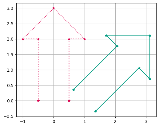
# These points describe an arrow
original_coordinates = np.array(
    [[-0.5, 0], [-0.5, 2], [-1, 2], [0, 3], [1, 2], [0.5, 2], [0.5, 0]]
)
original_coordinates = original_coordinates.transpose()

# We need the x coordinates in one array and the same for y
orig_x = original_coordinates[0, :]
orig_y = original_coordinates[1, :]

number_of_points = len(orig_x)

ones = np.ones((1, number_of_points))  # should have the same dimension as orig_x

# This is how we go from normal 2D coordinates to homogeneous coordinates
homogenous_coordinates = np.vstack((orig_x, orig_y, ones))

# Now we perform the actual transformation by multiplying H with the homogeneous coordinates
transformed_coordinates = H @ homogenous_coordinates

# We need the x coordinates in one array and the same for y
transformed_x = transformed_coordinates[0, :]
transformed_y = transformed_coordinates[1, :]

# Draw the original arrow shape and the transformed shape
fig, ax = plt.subplots()

ax.plot(orig_x, orig_y, color="#db0651", marker="*", linestyle=":")
ax.plot(transformed_x, transformed_y, color="#009c82", marker="*")

# Format the figure
ax.grid(True)
ax.set_aspect("equal")

6.7. Exercises

To edit the code and run the code on the server, click the button to launch this page on JupyterHub. You can scroll down to the code, make changes, and run the cell with the play button.

6.7.1. Exercise 1

Make the arrow point downwards. Which parameter(s) did you change and what value(s) did you enter?

6.7.2. Exercise 2

Experiment with the parameters in the code (phi, tx and ty) to find out which point the coordinates are transformed around. I.e. which is the center point of the rotation?

6.7.3. Exercise 3

Can you rotate the arrow in such a way that the rotation is around the point (1,2)? Which parameter(s) did you change and what value(s) did you enter?

6.7.4. Exercise 4

What happens when you change the Math.cos and Math.sin parts of the H matrix?