5.2. Pinhole Camera Model

In order to estimate the unknown parameters of a camera, we need to describe (model) the system mathematically. This this chapter, we focus on having a mathematical model of the camera.

Imagine standing in front of a landscape, closing one eye, and holding up a small rectangular frame. The scene projects through that frame as if the world were painted onto a flat surface. That’s exactly how a camera perceives its environment, it maps points from the 3D world onto a 2D image plane through a process of projection.

But unlike our eyes, a camera’s geometry is not innate; we have to model it mathematically. That’s what a camera model does. It tells us:

• How a 3D point projects into an image (the forward projection), and

• How we can recover a 3D ray or point from an image pixel (the back-projection).

In this chapter, we focus on the pinhole camera model, the foundational model in computer vision and robotics. It’s simple yet remarkably powerful and it’s the basis for most modern camera systems, even those that later add lens distortion or fisheye extensions.

Specifically, we will learn about

• Intrinsic parameters

• Extrinsic parameters

• The complete camera projection matrix

5.2.1. Prerequisites

Note

Before reading this chapter you should be comfortable with matrices, vectors, homogeneous transformations, and basic concepts of linear algebra. See chapter Algebra & Calculus for a primer on these foundations.

5.2.2. Pin Hole Model

The concept of the Camera Obscura dates back thousands of years. If you place a small hole in the wall of a darkened room, light rays from the outside world pass through the hole and project a dim, inverted image onto the opposite wall. This simple but fascinating phenomenon is the foundation of all modern imaging and was first described in the 5th century by the Chinese philosopher Mozi, who observed that an inverted image of the world forms through a small aperture.

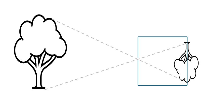
Fig. 5.2 Visualization of pinhole camera. The tree on the left is projected through the pinhole on the backplate of the camera on the right.

In a pinhole camera, only a tiny fraction of the light emitted or reflected by an object reaches the image plane through the small opening. Because there is no lens involved, the camera cannot adjust focus. Yet, interestingly, everything appears in focus regardless of the object’s distance from the hole. The trade-off is brightness: smaller holes yield sharper but darker images, while larger holes allow more light but introduce blur.

Modern digital cameras operate on the same fundamental principle but replace the pinhole with a lens. The lens focuses incoming light onto an image sensor, a semiconductor chip made up of millions of light-sensitive elements, which converts the light into a digital image. Whether in a camera or the human eye, image formation is a process of projection: a three-dimensional world is mapped onto a two-dimensional surface. In this transformation, depth information is lost, meaning we can no longer distinguish whether an image shows a large distant object or a small nearby one. This mapping from 3D to 2D is called perspective projection. This mapping from the 3-dimensional world to a 2-dimensional image has consequences that we can see below in Fig. 5.3:

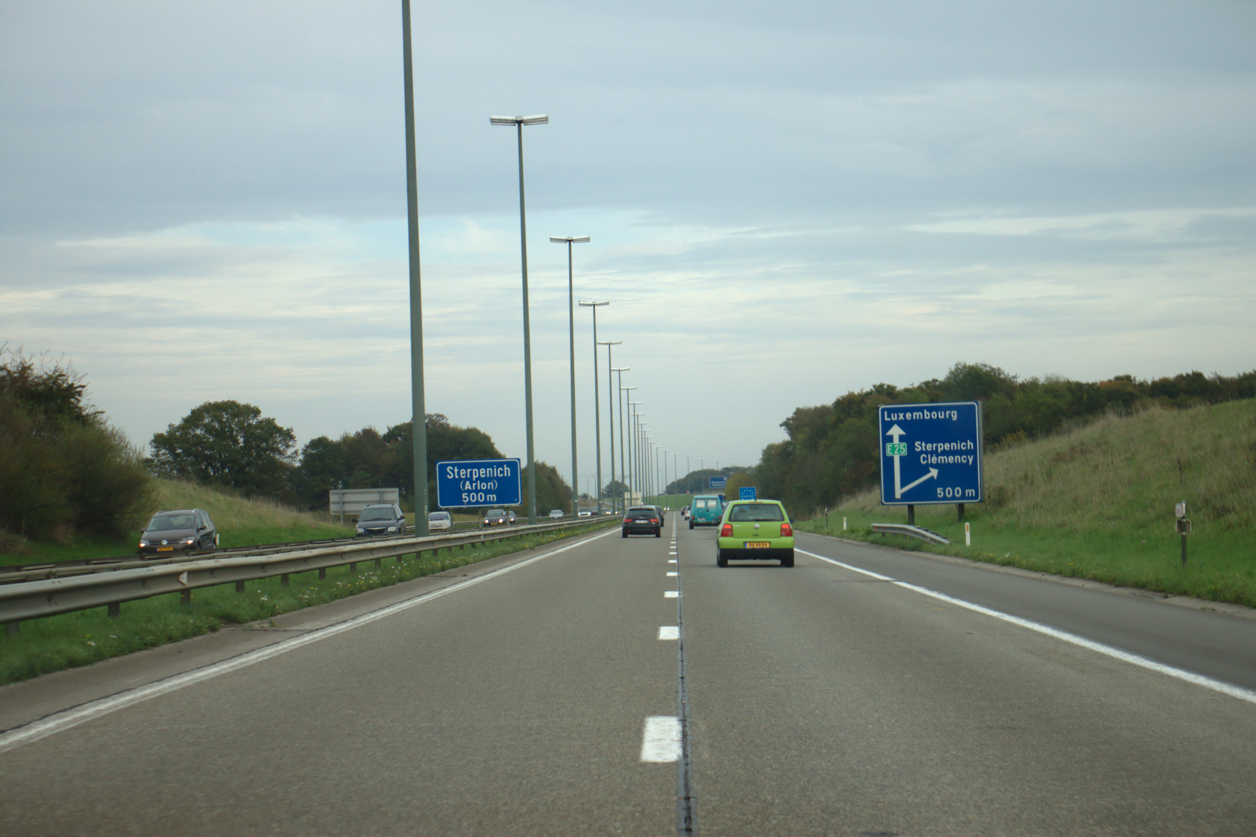
Fig. 5.3 Perspective Projection of highway (CC BY 3.0 https://commons.wikimedia.org/wiki/File:Sterpenich,_dálnice_A4.jpg)

In the figure, you see that parallel lines (the sides of the road) all point to one direction and are not parallel in the image. It is interesting that the parallel lines of the light poles are parallel in the picture. More formally, we can describe the transformation from the 3D world to the 2D image plane as having the following properties:

1. Dimensionality reduction: The projection defines a mapping from three-dimensional space to a two-dimensional plane, expressed as \(P: \mathbb{R}^3 \rightarrow \mathbb{R}^2\)

2. Linearity of projections: Straight lines in the world are mapped to straight lines in the image. This mapping is a property of the projective transform.

3. Vanishing points and perspective: Parallel lines in the real world appear to converge at a single point on the image, known as the vanishing point. The only exception occurs when the lines are fronto-parallel (i.e., lying in a plane parallel to the image plane), then they remain parallel in the projection.

4. Projection of curves: Conic sections (family of curves obtained by the intersection of a plane with a cone) in 3D space are projected as conic sections in the image. For instance, a circular object may appear as either a circle or an ellipse depending on its orientation relative to the camera.

5. Scale distortion: The apparent size (or area) of an object is not preserved and varies with distance. Objects farther from the camera appear smaller.

6. Ambiguity of depth: The mapping is not one-to-one, meaning it has no unique inverse. Given an image point \(P_i = (x_i,y_i)\) we cannot uniquely determine its corresponding world point \(P_w = (x_w,y_w,z_w)\); all we can infer is that the 3D point must lie somewhere along the projection ray passing through \((x,y)\).

7. Non-conformality: The transformation is not conformal,i.e. it does not preserve shapes or internal angles. Unlike rigid transformations such as translation, rotation, or uniform scaling, perspective projection distorts the geometry of objects depending on their position and depth.

Mathematically, the pin hole model defines this projection from a point \(P_w\) in the 3D world coordinate frame to a point \(P_i\) in the image coordinate frame as described in equation equation (5.1)

(5.1)\[ P_i = K T_{cw}P_w \]

where

• \(K\) is the intrinsic camera matrix,

• \(T_{cw}\) is the extrinsic matrix, i.e. the homogeneous transformation from the world frame to the camera frame.

This compact equation, using concepts from linear algebra, might look complex and it hides a lot of meaning. So, let’s unpack it!

5.2.3. Intrinsic Parameters: How the camera projects

Intrinsic parameters are the innate characteristics of the camera and sensor. As such, they describe the internal geometry and optical characteristics of a camera that affect how 3D points in the camera’s coordinate system are projected onto its 2D image plane.

These parameters are typically represented in a camera intrinsic matrix \(K\), which captures the following key quantities:

(5.2)\[\begin{split} K = \begin{bmatrix} f_x & \alpha & u_x\\ 0 & f_y & v_y\\ 0 & 0 & 1\\ \end{bmatrix} \end{split}\]

where

• \(f_x, f_y\): The focal lengths in pixels along the \(x\) and \(y\) axes.

• \(\alpha\): The skew coefficient, accounting for non-rectangular pixels or the non-orthogonality between the image x- and y-axes. Nowadays most modern cameras have a negligibal skew, hence we assume \(\alpha = 0\).

• \(u_x, v_y\): The principal point, which is the projection of the camera’s optical center onto the image plane (expressed in pixels). It is typically near the center of the image.

Together, the intrinsic parameters define how the camera maps 3D points (in camera coordinates) to 2D pixel coordinates, independent of the camera’s position or orientation in the world. Let’s dive into the mathematics of this matrix in the next section and explain what all these terms mean.

5.2.3.1. Geometry of Image Formation

Image formation refers to how a lens bends (refracts) light rays from an object so that they converge and create an image. A thin convex lens forms images by bringing incoming light rays to a focus. The 2D cross-sectional diagram in Fig. 5.4 shows this process and the geometry behind it.

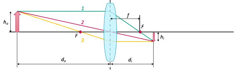
Fig. 5.4 Image formation geometry (source: Machine Vision Design course of SMART).

In the figure above, the lens features two focal points, each placed at a distance \(f\) on opposite sides. In addition, the d-coordinate of the object is measured from the center of the lens, as described by the thin lens equation:

(5.3)\[ \frac{1}{d_o} + \frac{1}{d_i} = \frac{1}{f} \]

where \(d_o\) is the distance to the object, \(d_i\) is the distance to the image, and \(f\) is the focal length of the lens. For \(d_o > f\) an inverted image is formed on the image plane at \(d_i < -f\).

While the thin lens equation describes how real lenses form images through refraction and focusing, many computer vision algorithms rely on a simplified geometric model of this process, the central perspective projection model illustrated in Fig. 5.5. Instead of modeling the physical lens in detail, this model approximates image formation as a projection of 3D points through a single central point onto an image plane. This abstraction captures the essential geometry of how a scene appears in an image, without the complexity of real optical systems.

In the central perspective projection model, light rays converge at the origin of the right-handed camera frame \(\{C\}\), and an non-inverted image is formed on the image plane positioned at \(z = f\). The z-axis intersects the image plane at the principal point, which is the origin of the 2D image coordinate system; because of this we also call the z-axis the optical axis.

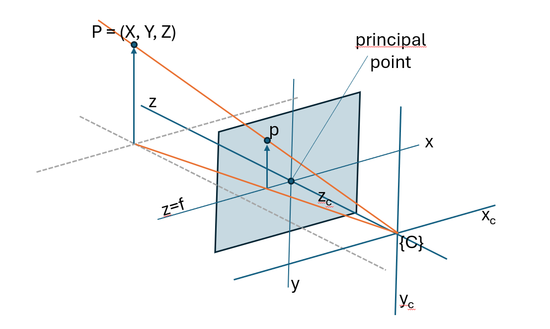
Fig. 5.5 Central perspective projection model.

By applying similar triangles and proportionality, a point in camera coordinates \(P_{c}=(x_{c},y_{c},z_{c})\) can be mapped to an image point \(P_{i}=(x_{i},y_{i})\) as described in equation (5.4):

(5.4)\[ x_{i}=f\frac{x_{c}}{z_{c}},y_{i}=f\frac{y_{c}}{z_{c}} \]

This mapping expresses the central characteristic of perspective projection: Although the final image coordinates include the focal length as a scaling factor, the essential geometric action of perspective projection depends only on the ratios \(\frac{x_{c}}{z_{c}}\) and \(\frac{y_{c}}{z_{c}}\). These ratios encode the direction of the 3D point relative to the camera, and is independent of the chosen focal length. In other words, geometrically, all points lying along the same 3D ray through the camera center project to the same 2D pixel.

Fig. 5.6 Points on the ray projecting to the same point on the image plane.

Note how this is exactly what homogeneous coordinates are designed to express: in homogeneous form, points that differ only by a scalar factor represent the same geometric entity, allowing the perspective projection, including its inherent scale ambiguity, to be written as a simple linear transformation followed by normalization.

Formally, a homogenous coordinate \(P_h\) augments an \(n\)-dimensional point \(P\) with an additional scale component \(s\), where often \(s = 1\) for simplicity (in case of \(s = 0\) we represent points “at infinity,” i.e., directions). For instance, for a 3D Cartesian point the mapping \(P \rightarrow P_H\) is

(5.5)\[\begin{split} \begin{bmatrix} x \\ y \\ z \\ \end{bmatrix} \rightarrow \begin{bmatrix} x \\ y \\ z \\ s \\ \end{bmatrix} \end{split}\]

For the inverse mapping, \(P_h \rightarrow P\), one divides all elements of the homogeneous vector by its last element, e.g. for a 3D homogeneous vector one gets its 2D cartesian counterpart by:

(5.6)\[\begin{split} \begin{bmatrix} x \\ y \\ z \end{bmatrix} \rightarrow \begin{bmatrix} \frac{x}{y} \\\frac{ y}{z}\end{bmatrix} \end{split}\]

if \(z \neq 0\). If \(z = 0\), the point lies at infinity, representing a direction rather than a finite Cartesian point.

Thus, we can write the image plane point coordinates described in equation (5.4) explicitly as homogeneous coordinates as

(5.7)\[ \tilde{x_i} = fx_c, \tilde{y_i} = fy_c,\tilde{ z_i} = z_c \]

This way, we can express a point \(P_c\) in the camera frame as

(5.8)\[\begin{split} P_i = K P_c \\ \end{split}\]

(5.9)\[\begin{split} \begin{bmatrix} \tilde{x_i} \\ \tilde{y_i} \end{bmatrix} = \begin{bmatrix} f & 0 & 0\\ 0 & f & 0\\ 0 & 0 & 1 \end{bmatrix} \begin{bmatrix} x_{c}\\ y_{c}\\ z_{c} \end{bmatrix} \end{split}\]

We can also explicitly express this scale ambuiguity by writing the image plane point as a non-homogeneous coordinate:

(5.10)\[\begin{split} s \begin{bmatrix} u\\ v\\ 1 \\ \end{bmatrix} = \begin{bmatrix} f & 0 & 0 \\ 0 & f & 0 \\ 0 & 0 & 1 \\ \end{bmatrix} \begin{bmatrix} x_{c}\\ y_{c}\\ z_{c} \end{bmatrix} \end{split}\]

where \(s = z_c\).

Note

The projection from 3D camera coordinates to 2D image coordinates expresses mathematically one crucial fact: we lose scale information.

This follows immediately from the homogeneous representation. The matrix multiplication above produces a homogeneous vector \((\tilde{x_i}, \tilde{y_i}, \tilde{z_i})\), and the final Cartesian image coordinates are obtained only after dividing by \(\tilde{z_i}\). Because homogeneous coordinates are defined up to an arbitrary nonzero scale factor, the following vectors all represent the same image point:

(5.11)\[\begin{split} \begin{bmatrix} f x_c \\ f y_c \\ z_c \end{bmatrix} \sim s \begin{bmatrix} f x_c \\ f y_c \\ z_c \end{bmatrix} \qquad \forall s \neq 0. \end{split}\]

This implies:

• Points \((x,y,z)\) and \(sx, sy, sz\) project to the same point in the image plane!

• Only the direction of the ray from the camera center is preserved; the absolute distance along that ray is discarded during the perspective divide.

• The image formation process therefore cannot recover metric depth from a single view.

Thus, this projection process loses absolute scale information: the camera cannot distinguish whether an object is small and close, or large and far away, if the projected angles are identical.

5.2.3.2. Skew

Next, there is one more parameter in \(K\) that we did not discuss yet, the skew parameter \(\alpha\).

\[\begin{split} K = \begin{bmatrix} f_x & \alpha & 0\\ 0 & f_y & 0\\ 0 & 0 & 1\\ \end{bmatrix} \end{split}\]

Up to this point, we assumed that the image axes are perfectly orthogonal, i.e. that the sensor’s pixel grid is rectangular, with the \(x\) and \(y\) axis forming a right angle. Modern cameras satisfy this assumption almost perfectly, which is why the “simplified” intrinsic matrix contains only the focal lengths \(f_x, f_y\) and the principal point \((c_x, c_y)\).

However, in the pinhole camera model, we allow for the possibility that the sensor axes are not perfectly perpendicular. This non-orthogonality is captured by the skew parameter \(\alpha\), which measures the angle between the image coordinate axes.

Fig. 5.7 Skewed pixel vs normalized pixel grid.

The skew coefficient is calculated as follows:

(5.12)\[ \alpha = f_x \tan(\theta) \]

where \(\theta\) is the angle between between the image plane axes. If \(\theta = 90^\circ\), then \(s = 0\).

By adding \(\alpha\) to our camera calibration matrix \(K\) as follows, we unskew and normalize the skewed image plane:

(5.13)\[\begin{split} K = \begin{bmatrix} f_x & \alpha & 0 \\ 0 & f_y & 0\\ 0 & 0 & 1\\ \end{bmatrix} \end{split}\]

See this blog post for more information of how one arrives to equations (5.12) and (5.13).

Should you care about skew?

You’ll be glad to hear that for most modern cameras, you can ignore axis skew entirely. Today’s CCD sensors are manufactured such that their pixel axes are perpendicular, i.e. \(\theta = 90^\circ\).

In practical situations, skew only becomes relevant in special cases, such as when you capture an image of another image. This can happen when re-photographing a print or enlarging a negative. For instance, if you enlarge a picture taken with a pinhole (film) camera using a lens whose optical axis isn’t perfectly perpendicular to the film or projection plane, a non-zero skew can appear. OpenCV actually omits the skew term altogether.

To sum up, you would need to account for axis skew when calibrating unusual cameras or cameras taking photographs of photographs, else you can happily ignore the skew parameter.

Reference: https://blog.immenselyhappy.com/post/camera-axis-skew/

5.2.3.3. Discrete Image Plane

Wait …

You might wonder, how can we express a point in the camera frame in pixels then? Let’s find out!

In a digital camera, the image plane consists of a \(\text{W} \times \text{H}\) array of light-sensitive units known as photosites, each directly corresponding to a pixel in the final image, as illustrated in Fig. 5.8. Pixel positions are represented by a 2D vector \((u,v)\) of nonnegative integers, with the origin placed by convention at the top-left corner of the image plane (see Fig. 5.9). Because of this convention, we need to add the translation from the center of the image plane to the top left corner in pixels, indicated by \(u_0\) and \(v_0\). Since the pixels are evenly sized and arranged on a regular grid, the pixel coordinates can be expressed via the image-plane coordinates as shown in equation equation (5.14):

(5.14)\[ u = \frac{x}{p_\text{W}} + u_0, v = \frac{y}{p_\text{H}} + v_0 \]

where \(p_\text{W}\) and \(p_\text{H}\) are the photosite dimensions, i.e. the width and height of each pixel respectively, and \((u_0,v_0)\) is the principal point, i.e. the pixel coordinate of the point where the optical axis intersects the image plane with respect to the new origin.

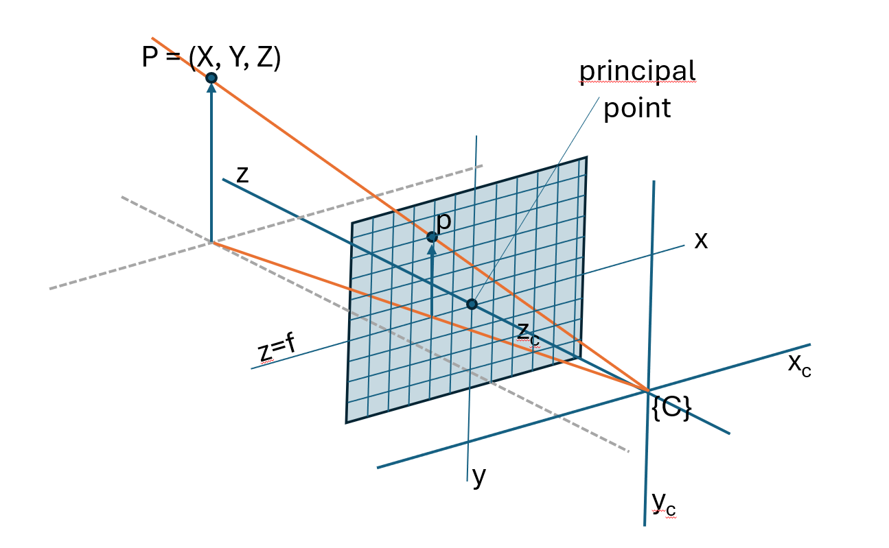
Fig. 5.8 Central perspective projection model on discrete grid.

Fig. 5.9 Origin of pixel coordinates vs image plane.

Using these parameters, we can express \(K\) in pixels as follows:

(5.15)\[\begin{split} K = \begin{bmatrix} 1/p_\text{W} & \alpha & u_0 \\ 0 & 1/p_\text{H} & v_0 \\ 0 & 0 & 1 \end{bmatrix} \begin{bmatrix} f & 0 & 0 \\ 0 & f & 0 \\ 0 & 0 & 1 \end{bmatrix} \end{split}\]

(5.16)\[\begin{split} K = \begin{bmatrix} f_x & \alpha & u_x\\ 0 & f_y & v_y\\ 0 & 0 & 1\\ \end{bmatrix} \end{split}\]

where

(5.17)\[ f_x = \frac{f}{p_\text{W}}, f_y = \frac{f}{p_\text{H}} \]

are the focal lengths in x and y direction expressed in pixels. Putting it together we can express a point in the camera frame in pixels as:

(5.18)\[\begin{split} P_i = \underbrace{ \begin{bmatrix} f_x & \alpha & u_0 \\ 0 & f_y & v_0 \\ 0 & 0 & 1 \end{bmatrix} }_K P_c \end{split}\]

5.2.3.4. Exercise 1: Intrinsic Parameters

Let’s put our new gained knowledge to the test!

In the code below can run an interactive demo on intrinsic parameters of the camera. Try the following:

• Changing the focal length values \(f_x\) and \(f_y\).

• Changing principal points \(u_x\) and \(u_v\).

• Changing the skew coefficient \(s\).

• How does changing the scale (or resolution) \(s\) affect the focal length and principal point?

Show code cell content

Hide code cell content

import numpy as np
import matplotlib.pyplot as plt
import ipywidgets as widgets
from ipywidgets import interact

# Tuneable Parameters
dist = 3
fx = 800
fy = 800
cx = 320
cy = 240
img_h = 800
img_w = 800
s = 0  # skew

# Generate synthetic 3D points in a simple 2D grid in front of the camera (Z = constant)
X, Y = np.meshgrid(np.linspace(-2, 2, 20), np.linspace(-2, 2, 20))
Z = np.ones_like(X) * dist  # points all at Z=3 meters
points_3D = np.stack([X.flatten(), Y.flatten(), Z.flatten()], axis=1)


def project_intrinsics(fx=800, fy=800, cx=320, cy=240, img_w=640, img_h=480, s=0):
    K = np.array([[fx, s, cx], [0, fy, cy], [0, 0, 1]])

    # Project
    proj = (
        K @ points_3D.T
    ).T  # points_3D has shape (N, 3). Transpose, so we can multiply by K, then transpose result back again.
    proj = (
        proj[:, :2] / points_3D[:, 2, np.newaxis]
    )  # Divide first 2 columns by third column -> Divide X and Y by Z to move from homogeneous coords to pixel coords.

    # Plotting
    plt.figure(figsize=(6, 5))
    plt.scatter(proj[:, 0], proj[:, 1], s=10)

    plt.xlim(0, img_w)
    plt.ylim(img_h, 0)
    plt.grid(True)
    plt.title(f"Z={dist}, fx={fx}, fy={fy}, cx={cx}, cy={cy}")
    plt.xlabel("u [px]")
    plt.ylabel("v [px]")
    plt.show()


project_intrinsics(fx, fy, cx, cy, img_w, img_h, s)

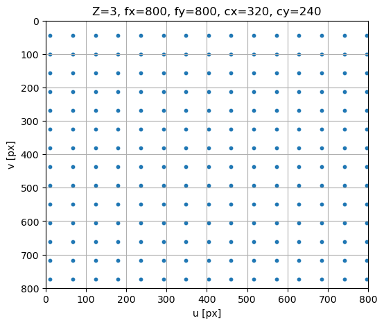
If you played if code above you might have noticed that …

• Changing the Z parameter will put the image at larger or smaller distance …

• Changing the focal length values \(f_x\) and \(f_y\) will zoom in or out …

• Changing the skew will tear the image …

• Changing principal points \(u_x\) and \(u_v\) will shift the distance

5.2.3.5. Extrinsic Parameters: Where the camera is in the world

Until now, we have been working with a point that is already expressed in the camera frame \(\{C\}\). Typically we will however work with points that are expressed in the world frame \(\{W\}\). The extrinsic parameters describe the rigid-body transformation between the world coordinate system and the camera’s coordinate system. This transform allows us to express any 3D world point in the camera frame and is expressed as follows:

(5.19)\[\begin{split} \begin{bmatrix} x_c \\ y_c\\ z_c\\ 1 \end{bmatrix} = \begin{bmatrix} R_{cw} & t_{cw} \\ 0 & 1 \end{bmatrix} \begin{bmatrix} x_w \\ y_w\\ z_w\\ 1 \end{bmatrix} \end{split}\]

or

(5.20)\[ P_c = T_{cw} P_w \]

where \(P_c\) is a homogeneous point expressed in frame \(\{C\}\), \(T_{cw}\) is the homogeneous transformation from frame \(\{W\}\) to frame \(\{C\}\) and \(P_w\) is a homogeneous point expressed in frame \(\{W\}\). Additionally, \(R_{cw}\) is a 3 \(\times\) 3 rotation matrix expressing the orientation of the camera and \(t_{cw}\) is a 3 \(\times\) 1 translation vector expressing the position of the camera in world coordinates.

Insert figure illustrating the equation above

Intuitively, \(R_{cw}\) and \(t_{cw}\) tell us where the camera is looking and from where. They connect the camera to the robot’s kinematics, for instance, mounting a camera on a robot arm or drone requires knowing its extrinsics relative to the robot frame. Only after transforming to the camera frame do we apply the pinhole projection.

Why do we need homogeneous coordinates for the extrinsic parameters?

A rigid-body transformation from frame \(a\) to frame \(b\) consists of a rotation followed by a translation:

(5.21)\[ P_b = R_{ba}P_a + t_{ba} \]

While rotation is a linear transformation, translation is affine and cannot be represented by a matrix multiplication in ordinary Euclidean coordinates. This makes it impossible to combine multiple rigid-body transformations into a single linear operator in Euclidian space \(\mathbb{R}^3\).

Homogeneous coordinates resolve this limitation by augmenting each point with a scale component \(s\): $\( \begin{bmatrix} x \\ y \\ z \\ \end{bmatrix} \rightarrow \begin{bmatrix} x \\ y \\ z \\ s \\ \end{bmatrix} \)$ (homogeneous_mapping_scale)

In case of rigid body transformation, we choose \(s = 1\).

If we want to express a translation of a vector as a matrix product, we can write:

(5.22)\[\begin{split} \begin{bmatrix} 1 & 0 & 0 & t_1 \\ 0 & 1 & 0 & t_2 \\ 0 & 0 & 1 & t_3 \\ 0 & 0 & 0 & 1 \\ \end{bmatrix} \begin{bmatrix} x \\ y \\ z \\ 1 \\ \end{bmatrix} \end{split}\]

and rotation around an angle \(\theta\) (here around the roll axis, i.e. the X axis) can be written as

(5.23)\[\begin{split} \begin{bmatrix} \cos(\theta) & -\sin(\theta) & 0 & 0 \\ sin(\theta) & \cos(\theta) & 0 & 0 \\ 0 & 0 & 1 & 0 \\ 0 & 0 & 0 & 1 \\ \end{bmatrix} \begin{bmatrix} x \\ y \\ z \\ 1 \\ \end{bmatrix} \end{split}\]

Together, rotation and translation can be expressed as one linear matrix \(T\):

(5.24)\[\begin{split} T = \begin{bmatrix} r_{11} & r_{12} & r_{13} & t_1 \\ r_{21} & r_{22} & r_{23} & t_2 \\ r_{31} & r_{22} & r_{33} & t_3 \\ 0 & 0 & 0 & 1 \\ \end{bmatrix} \end{split}\]

where \(R_{ij}\) represents the elements of a general \(3\times 3\) 3D rotation matrix, i.e. \(R = R_z(\phi) R_y(\beta) R_x(\theta)\) with the yaw, pitch and roll angles \(\phi\), \(\beta\) and \(\theta\) respectively.

In a more compact form we can write it as

(5.25)\[\begin{split} T_{ba} = \begin{bmatrix} R_{ba} & t_{ba} \\ 0 & 1 \end{bmatrix} \end{split}\]

As such, this representation has the major advantage that we can express rotation and translation in one single matrix, allowing us to chain transformations between multiple frames.

Moreover, the camera intrinsics operate on the same principle. The mapping from normalized image coordinates to pixel coordinates includes not only linear operations (scaling and shearing) but also a translation by the principal point. Just as with rigid-body motion, this translation term prevents the intrinsic mapping from being represented as a purely linear operator in Euclidean coordinates. Thus, by switching to homogeneous coordinates, this affine mapping becomes linear and we can express all rotation, translation and shearing operations as a compact sequence of linear transformations.

Note that we need to refactor \(K\), since \(P_c\) is now also a homogeneous point and thus a 4 \(\times\) 1 vector:

(5.26)\[\begin{split} K = \begin{bmatrix} f_x & \alpha & u_0 \\ 0 & f_y & v_0 \\ 0 & 0 & 1 \end{bmatrix} \begin{bmatrix} 1 & 0 & 0 & 0 \\ 0 & 1 & 0 & 0\\ 0 & 0 & 1 & 0 \end{bmatrix} \end{split}\]

Putting everything together, we can write equation (5.27) as

(5.27)\[\begin{split} s \underbrace{ \begin{bmatrix} u \\ v \\ 1 \end{bmatrix} }_{P_i} = \underbrace{ \begin{bmatrix} f_x & \alpha & u_0 \\ 0 & f_y & v_0 \\ 0 & 0 & 1 \end{bmatrix} \begin{bmatrix} 1 & 0 & 0 & 0 \\ 0 & 1 & 0 & 0\\ 0 & 0 & 1 & 0 \end{bmatrix} }_K \underbrace{ \begin{bmatrix} R_{cw} & t_{cw} \\ 0 & 1 \end{bmatrix} }_{T_{cw}} \underbrace{ \begin{bmatrix} x_w \\ y_w\\ z_w\\ 1 \end{bmatrix} }_{P_w} \end{split}\]

5.2.3.6. Exercise 2: Extrinsic Parameters

Let’s put our new gained knowledge to the test!

In the code below can run an interactive demo on extrinsic parameters of the camera. Try the following:

• Translating t along Z moves the camera closer or farther from the scene.

• Try to change \(R\) to tilt or pan the scene.

• Try changing the coordinate of the \(P_w\) itself vs translating and rotating it.

# Intrinsic Parameters
dist = 3
fx = 800
fy = 800
cx = 320
cy = 240
img_h = 800
img_w = 800
s = 0  # skew

# Extrinsic parameters
# Translation on [x,y,z] in meters
t_x = 0
t_y = 0
t_z = 5

# Rotation components in degrees
yaw = 0
roll = 0
pitch = 0

# Generate synthetic 3D points in a simple 2D grid in front of the camera (Z = constant)
X, Y = np.meshgrid(np.linspace(-2, 2, 20), np.linspace(-2, 2, 20))
Z = np.ones_like(X) * dist  # points all at Z=3 meters
points_3D = np.stack([X.flatten(), Y.flatten(), Z.flatten()], axis=1)


def project_intrinsics_and_extrinsics(
    fx=800,
    fy=800,
    cx=320,
    cy=240,
    img_w=640,
    img_h=480,
    s=0,
    t_x=0,
    t_y=0,
    t_z=0,
    yaw=0,
    roll=0,
    pitch=0,
):
    # Extrinsic
    # Roll (rotate around Z)
    roll_rad = np.radians(roll)
    R_roll = np.array(
        [
            [np.cos(roll_rad), -np.sin(roll_rad), 0],
            [np.sin(roll_rad), np.cos(roll_rad), 0],
            [0, 0, 1],
        ]
    )

    # Pitch (rotation around X)
    pitch_rad = np.radians(pitch)
    R_pitch = np.array(
        [
            [1, 0, 0],
            [0, np.cos(pitch_rad), -np.sin(pitch_rad)],
            [0, np.sin(pitch_rad), np.cos(pitch_rad)],
        ]
    )

    # Yaw (rotation around Z)
    yaw_rad = np.radians(yaw)
    R_yaw = np.array(
        [
            [np.cos(yaw_rad), 0, np.sin(yaw_rad)],
            [0, 1, 0],
            [-np.sin(yaw_rad), 0, np.cos(yaw_rad)],
        ]
    )

    # Compose 3D rotation
    R = R_yaw @ R_pitch @ R_roll

    # Build 4×4 homogeneous rigid body transformation matrix
    T = np.eye(4)
    T[:3, :3] = R
    T[:3, 3] = np.array([t_x, t_y, t_z])

    # Convert 3D world points to homogeneous points
    points_h = np.hstack([points_3D, np.ones((points_3D.shape[0], 1))])  # Nx4

    # Apply extrinsic transformation
    pts_cam_h = (T @ points_h.T).T  # Nx4

    # Check that we have positive Z in the camera frame
    valid = pts_cam_h[:, 2] > 0
    pts_cam_h = pts_cam_h[valid]

    # 3x4 intrinsic camera matrix
    K_ext = np.array([[fx, s, cx, 0], [0, fy, cy, 0], [0, 0, 1, 0]])

    p_h = (K_ext @ pts_cam_h.T).T  # Nx3 homogeneous pixel coordinates
    u = p_h[:, 0] / p_h[:, 2]
    v = p_h[:, 1] / p_h[:, 2]

    # Plotting
    plt.figure(figsize=(6, 5))
    plt.scatter(u, v, s=10)

    plt.xlim(0, img_w)
    plt.ylim(img_h, 0)
    plt.grid(True)
    plt.title(
        f"4×4 Extrinsic + Extended 3×4 Intrinsic Projection\n"
        f"roll={roll}°, pitch={pitch}°, yaw={yaw}°\n"
        f"t = ({t_x}, {t_y}, {t_z})"
    )
    plt.xlabel("u [px]")
    plt.ylabel("v [px]")
    plt.show()


project_intrinsics_and_extrinsics(
    fx, fy, cx, cy, img_w, img_h, s, t_x, t_y, t_z, yaw, roll, pitch
)

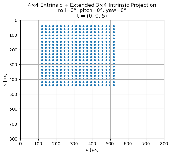
If you played if code above you might have noticed that …

• We roll around the Z axis (rotate the image), pitch around the X axis (tilt up/down) and yaw around the Y axis (turn left/right), instead of rolling around the X axis, pitching around the Y axis and yawing around the Z axis. This is because of the convention of the camera coordinate system where X = Right, Y = Down, Z = Forward.

5.2.3.7. The Complete Projection Equation

In summary, the pin hole camera model described by equation (5.28) combines extrinsic and intrinsic parameters to map 3D points in the world to 2D pixel locations on the image plane.

(5.28)\[\begin{split} s \underbrace{ \begin{bmatrix} u \\ v \\ 1 \end{bmatrix} }_{P_i} = \underbrace{ \begin{bmatrix} f_x & \alpha & u_0 & 0\\ 0 & f_y & v_0 & 0\\ 0 & 0 & 1 & 0 \end{bmatrix} }_K \underbrace{ \begin{bmatrix} R_{cw} & t_{cw} \\ 0 & 1 \end{bmatrix} }_{T_{cw}} \underbrace{ \begin{bmatrix} x_w \\ y_w\\ z_w\\ 1 \end{bmatrix} }_{P_w} \end{split}\]

Here, the extrinsic parameters describe the pose of the camera in the world: a rotation that aligns the world axes with the camera axes, and a translation that specifies the camera’s position. Together, they form a homogeneous transformation that converts world-frame points into the camera frame.

Once points are expressed in the camera coordinate system, the intrinsic parameters determine how these coordinates are projected onto the image sensor. The intrinsic matrix encodes the focal lengths, principal point, and skew, converting normalized camera rays into pixel coordinates based on the camera’s internal geometry.

By combining both components into a single projection pipeline, the model provides a complete mathematical description of image formation. This framework is fundamental for tasks such as 3D reconstruction, pose estimation, and sensor fusion, and serves as the basis for all further reasoning about geometric perception in computer vision and robotics.

Attention

The camera projection model (equation (5.28)) includes several parameters that are typically unknown in practice. The principal point is often not exactly at the center of the photosite array, and the focal length of a lens can deviate by up to about 4% from its specified value, being strictly correct only when the lens is focused at infinity. It is also well known that the intrinsic parameters can vary when a lens is removed and reattached or when its focus or aperture is adjusted.

Generally, the only intrinsic quantities that can be reliably obtained are the photosite dimensions \(p_\text{W}\) and \(p_\text{H}\), which are usually available in the sensor manufacturer’s specifications.

This is why we need to calibrate the camera!

Attention

Note that the equation above only describes an ideal pinhole camera model, that is, there is no distortion included in this model.

"""
Insert exercises:
* Apply intrinsic camera matrix to a real image instead of synthetic points.
* Create a point cloud from depth image using intrinsic and extrinsic parameters.
* Apply some intrinsic parameters to a distorted camera image → could be a nice transition to next chapter, Distortion. For now, the Distortion chapter is out of scope due to time.
"""

'\nInsert exercises:\n* Apply intrinsic camera matrix to a real image instead of synthetic points.\n* Create a point cloud from depth image using intrinsic and extrinsic parameters.\n* Apply some intrinsic parameters to a distorted camera image → could be a nice transition to next chapter, Distortion. For now, the Distortion chapter is out of scope due to time.\n'