Vector space

6.1. Vector space#

For a set of elements to be called a vector space \(\mathcal{V}^n\), it must comply to a few conditions:

Addition: It’s elements may be added to each other, and the result is part of the same space;
Scalar multiplication: It’s elements may be multiplied by a scalar (generally a real-valued number, but can also be complex) and the result is part of the same space;
An origin: There must be a single element in the set that is the absolute reference, \(o\in\mathcal{V}^n\).

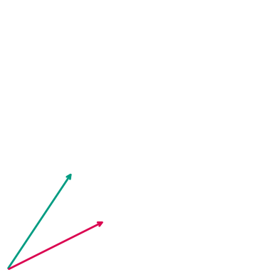
The simplest vector space is \(\mathcal{V}\), the space of one-dimensional vectors. A more intuitive vector space is \(\mathcal{V}^2\), which can be better visualized on a page or display. Addition in \(\mathcal{V}^2\) can be visualized as follows:

vector_sum — Fig. 6.1 Addition of the green and the pink vectors, visualized as arrows, results in the blue vector.#

The blue vector in Fig. 6.1 also starts from the same point, the origin.

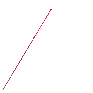
Scalar multiplication in \(\mathcal{V}^2\) can be visualized as follows:

Notice how these operations are valid even without expressing the vectors using numbers. Vectors are geometric entities, like planes, lines, points, etc.

In this part of this work we use real vector spaces.

6.1.1. Euclidean spaces#

Vector spaces do not have an inner product operation in general. The vector spaces that do, are a subset of all vector spaces often referred to as Euclidean spaces or inner product spaces.

For Euclidean spaces, the inner product is a mapping from two vectors to a real number. This inner product gives us the tools to do some more operations in Euclidean space:

Inner product:

\[ \InnerProduct{}{}:\mathcal{E} \times \mathcal{E} \rightarrow \mathbb{R} \]
Norm (distance, also two-norm):

\[ \lVert \ldots \rVert_{2}:\mathcal{E} \rightarrow \mathbb{R} \]

Defined for a vector \(v\) as:

\[ v \rightarrow \sqrt{\InnerProduct{v}{v}} \]
Angle between two vectors:

\[ v \angle w = \arccos\left(\frac{\InnerProduct{v}{w}}{\lVert v \rVert_{2}\cdot\lVert w \rVert_{2}}\right) \]
Orthogonality of two vectors:

\[ v \perp w \Leftrightarrow \InnerProduct{v}{w} = 0 \]

This set of operations provides us with the ability to relate lengths and angles of different vectors. But we still don’t have numbers to express vectors, so all operations can only be done by drawing. If we want computers to apply these operations however, we have to express vectors in numbers.

To do that, for some \(n\)-dimensional Euclidean space, we define \(n\) unit base vectors \(e_1,\ldots,e_n\) which are all mutually orthogonal and unit length. Together, we call these the base or basis[1], and because the base vectors are orthogonal and unit length, we call such a base an orthonormal basis. Taking \(\mathcal{E}^2\) as example, we define two perpendicular base vectors \(e_1\) and \(e_2\).

Using a base allows us to map vectors to numbers, because we define the base vectors as follows:

\[\begin{split} \begin{aligned} e_1 = \begin{bmatrix} 1 \\ 0 \end{bmatrix}, \quad e_2 = \begin{bmatrix} 0 \\ 1 \end{bmatrix} \end{aligned} \end{split}\]

Because the result of scalar multiplication and vector addition is still in the same vector space, we can use a linear combination of the base vectors to express other vectors in the same space. So for a generic vector \(v\in\mathcal{E}^2\) that would be:

\[\begin{split} \begin{aligned} v &= x e_1 + y e_2 = x \begin{bmatrix} 1 \\ 0 \end{bmatrix} + y \begin{bmatrix} 0 \\ 1 \end{bmatrix} \\ &= \begin{bmatrix} 1 & 0 \\ 0 & 1 \end{bmatrix} \begin{bmatrix} x \\ y \end{bmatrix} \\ &= \begin{bmatrix} x \\ y \end{bmatrix} \end{aligned} \end{split}\]

Where \(x\) and \(y\) are real-valued scalars. This can be generalized to \(n\)-dimensional Euclidean spaces:

\[\begin{split} v \in \mathcal{E}^n \rightarrow v = \begin{bmatrix} x_1 \\ x_2 \\ \vdots \\ x_n \end{bmatrix} \end{split}\]

Now that we have numeric representations of vectors in Euclidean space, we can also define how to calculate the inner product, which yields a scalar value indicating the similarity between the two vectors.

\[ \InnerProduct{v}{w} = v\Transposed w \]

6.2. Exercises#

from matplotlib import pyplot as plt
import numpy as np

from spf_settings import SAXION_COLS


def create_arrow_plot(xlim=(0, 4), ylim=(0, 4), xticks=[], yticks=[], **kwargs):
    return plt.axes(
        aspect="equal",
        frame_on=False,
        xlim=xlim,
        ylim=ylim,
        xticks=xticks,
        yticks=yticks,
        **kwargs,
    )


def arrow(ax, end, start=(0, 0), color=(0, 0, 0), dashed=False):
    ax.annotate(
        "",
        xy=end,
        xytext=start,
        arrowprops=dict(arrowstyle="->", color=color, lw=2, ls="--" if dashed else "-"),
    )

6.2.1. Exercise 1#

Recreate the figure shown above that demonstrates vector addition.

ax = create_arrow_plot()

v1 = np.array([[1], [1.5]])
v2 = np.array([[1.5], [0.75]])
# v3 = ?

arrow(ax, start=(0, 0), end=v1, color=SAXION_COLS.GREEN, dashed=False)
arrow(ax, start=(0, 0), end=v2, color=SAXION_COLS.PINK, dashed=False)

../_images/d4bbd3c8ef8a3bbcc1f0c810d681fa5071bdf5a35bf265568c4a16dce1385331.png

6.2.2. Exercise 2#

Recreate the figure shown above that demonstrates vector scalar multiplication.

ax = create_arrow_plot()

v1 = np.array([[1.5], [2.5]])

alpha = 1.5

# v2 = ?

arrow(ax, start=(0, 0), end=v1, color=SAXION_COLS.GREEN)

../_images/ca852c2c0fd58875348c86ff616f243198ecfd4c82b8b7427d81f9b76ca637e8.png

6.2.3. Exercise 3#

A certain vector is defined as \(v' = [1, 2, 3]^{\mathsf{T}}\), expressed in the following not so convenient base vectors:

\[\begin{split} e'_1 = \begin{bmatrix} 1 \\ 0 \\ 1 \end{bmatrix},\quad e'_2 = \begin{bmatrix} 0 \\ 1 \\ -1 \end{bmatrix}, \quad e'_3 = \begin{bmatrix} -1 \\ -1 \\ 0 \end{bmatrix} \end{split}\]

How would this vector be expressed in the more convenient orthogonal unit-length base vectors?

e1_prime = np.array([[1, 0, 1]]).T
# e2_prime = ?
# e3_prime = ?
# v_prime = ?

# v = ?