%matplotlib inline

import numpy as np
import matplotlib.pyplot as plt

from matplotlib import animation
from IPython.core.display import HTML
from scipy.optimize import minimize, OptimizeResult
import plotly.graph_objects as go


np.set_printoptions(precision=None, suppress=None)

7.1. Optimization

7.1.1. Introduction

In this notebook we will explore various optimization methods. On of the preliminaries are:

• calculus

In the context of sensing and perception, optimization is a real workhorse that is used in many algorithms. With optimization we refer to optimizing a function, that is, find the parameters that maximize (or minimize) this function. In general, this procedure is an iterative proces.

A typical use case is a calibration procedure where you want to optimize certain model paraemeters such that a systematic error can be ‘calibrated away’.

In Maximum Likelihood Estimation we use it to optimize the likelihood function.

All machine learning algorithm make use of some optimization technique to find the optimal parameters during the training phase.

Hence, often the function that is considered represents some cost or risk that has to be minimized.

A good starting point is a quadratic cost:

\[ f (x) = \frac{1}{2} x^T A x - b^T x \]

# Define A and b

A = np.array([[17, 2], [2, 7]])
b = np.array([2, 2])

x_true = np.linalg.solve(A, b)

# Define f(x)


def f(x):
    x1, x2 = x

    # Quadratic example
    f_func = lambda x: 0.5 * x.T @ A @ x - b.T @ x

    # Ensure that input array's / mesh is handled properly (used for surface)
    if type(x1) is np.ndarray:
        f = np.zeros_like(x1)

        for i, (x1i, x2i) in enumerate(zip(x1, x2)):
            for j, (x1ij, x2ij) in enumerate(zip(x1i, x2i)):
                x = np.array([x1ij, x2ij])

                f[i, j] = f_func(x)

    else:
        x = np.array([x1, x2])
        f = f_func(x)

    return f

s = 0.16
xmin, xmax = x_true[0] - s, x_true[0] + s
ymin, ymax = x_true[1] - 2 * s, x_true[1] + s


xi = np.linspace(xmin, xmax, 30)
yi = np.linspace(ymin, ymax, 30)
contourInterval = 1

X, Y = np.meshgrid(xi, yi)

Z = f([X, Y])

fig = go.Figure(
    go.Surface(
        x=xi[::contourInterval],
        y=yi[::contourInterval],
        z=Z[::contourInterval, ::contourInterval],
    )
)

fig.update_traces(
    contours_z=dict(
        show=True, usecolormap=True, highlightcolor="limegreen", project_z=True
    )
)

fig.update_layout(
    title="Arbitrary function with two inputs",
    autosize=False,
    width=800,
    height=800,
    margin=dict(l=100, r=100, b=100, t=90),
)

fig.show()

7.1.2. Descent methods

A large category of algorithms are the descent methods which is given by the following pseudocode:

**Inputs:** Given a function $f$ and initial value $x_0$.

**Output:** Calculate the value of $x$ that minimizes $f$.

- while *stopping criterium is not satisfied*: 
    1. Determine a descent direction $p$
    2. Line search: choose a step size $\alpha>0$
    3. Update: $x := x + \alpha p$

7.1.2.1. Gradient Descent (Steepest Ascent)

The most famous descent algorithm is the gradient descent (GD) method. The GD algorithm seeks for a minimum by setting the search direction iteratively to the negated gradient evaluated at the actual function value.

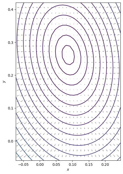
We start with visualizing the gradient of the function at a meshgrid of function values.

7.1.2.1.1. Exercise:

• Define the gradient of f as function of x and y

Show code cell content

Hide code cell content

# Answer


def gradient_f(xy):
    x1, x2 = xy

    gradient_f_func = lambda x: A @ x - b

    # Handle mesh inputs correctly
    if type(x1) is np.ndarray:
        grad = np.zeros((2, *x1.shape))

        for i, (x1i, x2i) in enumerate(zip(x1, x2)):
            for j, (x1ij, x2ij) in enumerate(zip(x1i, x2i)):
                x = np.array([x1ij, x2ij])

                grad[:, i, j] = gradient_f_func(x)
    else:
        x = np.array([x1, x2])
        grad = gradient_f_func(x)

    return grad

# Plot the vector field that represents the gradient at various positions
f0 = f(x_true)
Nlevels = 25
contourLevels = (np.linspace(f0, 1, Nlevels) - f0) ** 2 + f0


grad_z = gradient_f([X, Y])

dZ_dX = grad_z[0][::contourInterval, ::contourInterval]
dZ_dY = grad_z[1][::contourInterval, ::contourInterval]

fig, ax = plt.subplots(figsize=(8, 8))

ax.contour(X, Y, Z, levels=contourLevels)  # contour the function values
ax.quiver(
    X[::contourInterval, ::contourInterval],
    Y[::contourInterval, ::contourInterval],
    dZ_dX,
    dZ_dY,
    alpha=0.5,
)  # plot the gradient as arrows

ax.set_xlabel("$x$")
ax.set_ylabel("$y$")

ax.set_aspect("equal", "box")
# plt.grid()

plt.show()

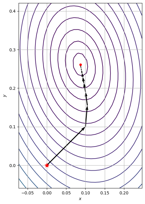
7.1.2.1.2. Exercise:

• Write your own gradient descent solver:

  • Define a stop criterium

  • Use a constant stepsize

  • Save the intermediate function values in a list path

• Evaluate the solutions for the following initial point: \(x_0 = [0, 0]\)

  • Use can use the function plotContourWithOptimizationPath

• Evaluate the solution for various stepsizes: \(\alpha \in \left(0, 1\right)\)

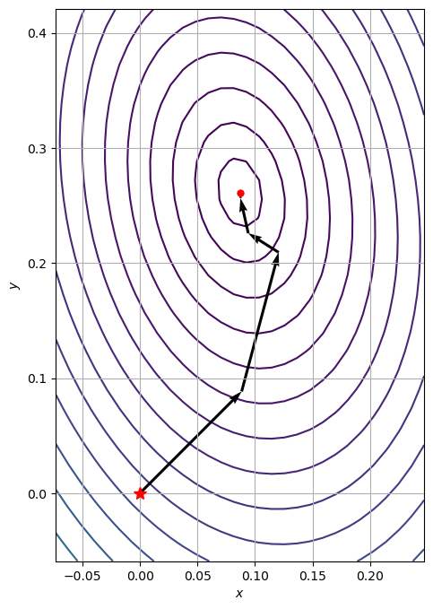
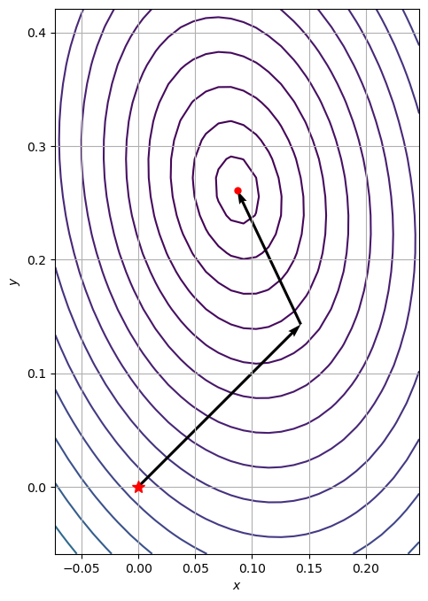
# Function to plot the traversed optimization path together with the function contour


def plot_contour_with_optimization_path(X, Y, Z, path_):
    path = np.array(path_).T

    fig, ax = plt.subplots(figsize=(8, 8))

    ax.contour(X, Y, Z, zorder=0, levels=contourLevels)
    ax.quiver(
        path[0, :-1],
        path[1, :-1],
        path[0, 1:] - path[0, :-1],
        path[1, 1:] - path[1, :-1],
        scale_units="xy",
        angles="xy",
        scale=1,
        color="k",
        zorder=1,
    )
    ax.plot(*x_true, "k.")
    ax.plot(*path[:, 0], "r*", markersize=10)
    ax.plot(*path[:, -1], "ro", markersize=5)

    ax.grid()
    ax.set_aspect("equal", "box")

    ax.set_xlabel("$x$")
    ax.set_ylabel("$y$")

Show code cell content

Hide code cell content

# answer

x0 = np.array([0.0, 0.0])
path_gd = [x0]

x_est = x0
alpha = 0.05

for i in range(1000):
    grad = gradient_f(x_est)
    if np.linalg.norm(grad) < 1e-5:
        gd = OptimizeResult(x=x_est, succes=True)
        print("Number of iterations: {}".format(i))
        print("Minimum: {}".format(x_est))
        print("Grad at minimum: {}".format(grad))
        break
    x_est = x_est - alpha * grad
    path_gd.append(x_est)

plot_contour_with_optimization_path(X, Y, Z, path_gd)

Number of iterations: 30
Minimum: [0.08695679 0.26086819]
Grad at minimum: [ 1.75687565e-06 -9.12272158e-06]

7.1.2.2. Line solver

A simple but effective and fast method to find the optimal step size (aka line solver) is backtracking line-search (Armijo’s rule).

7.1.2.2.1. Exercise:

• Replace the fixed step size with the backtracking line-search method.

  • The algorithm can be found at: Wikipedia: Backtracking line search

  • Use the normalized gradient for the search direction \(p\)

Show code cell content

Hide code cell content

# Answer

x_est = x0
tau = 0.5
c = 0.5

path_gd_ls = [x0]

for i in range(1000):
    grad = gradient_f(x_est)
    p = -grad  # Search direction
    grad_norm = np.linalg.norm(grad)
    grad_normalized = grad / grad_norm

    p = -grad_normalized
    m = grad.T @ p

    t = -c * m

    # Backtracking line solver part
    alpha = 1
    while f(x_est) - f(x_est + alpha * p) < alpha * t:
        alpha *= tau

    if grad_norm < 1e-5:
        print("Number of iterations: {}".format(i))
        print("Minimum: {}".format(x_est))
        print("Grad at minimum: {}".format(grad))
        break
    x_est = x_est + alpha * p
    path_gd_ls.append(x_est)

plot_contour_with_optimization_path(X, Y, Z, path_gd_ls)

Number of iterations: 14
Minimum: [0.08695666 0.26086858]
Grad at minimum: [ 4.02164958e-07 -6.59443897e-06]

There are some computational disadvantages with gradient descent. A more efficient method is the conjugate descent method which can be found in the scipy optimize library:

def make_minimize_cb(path=[]):
    def minimize_cb(xk):
        # note that we make a deep copy of xk
        path.append(np.copy(xk))

    return minimize_cb


path_cg = [x0]

res = minimize(
    f, x0=x0, method="CG", jac=gradient_f, tol=1e-20, callback=make_minimize_cb(path_cg)
)

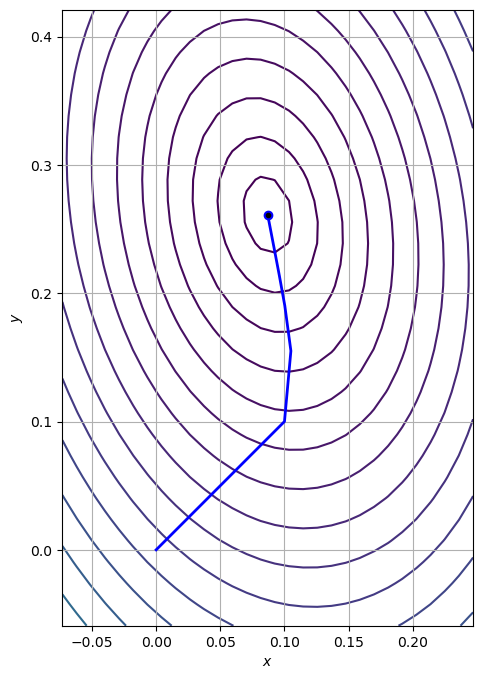
plot_contour_with_optimization_path(X, Y, Z, path_cg)

The trajectory can be animated using matplotlib’s FuncAnimation:

path = np.array(path_gd).T

fig, ax = plt.subplots(figsize=(8, 8))

ax.contour(X, Y, Z, zorder=0, levels=contourLevels)

(line,) = ax.plot([], [], "b", lw=2)
(point,) = ax.plot([], [], "bo")

ax.plot(*x_true, "k.")

ax.grid()
ax.set_aspect("equal", "box")

ax.set_xlabel("$x$")
ax.set_ylabel("$y$")


def init():
    line.set_data([], [])
    point.set_data([], [])
    return line, point


def animate(i):
    line.set_data(*path[::, :i])
    point.set_data(*path[::, i - 1 : i])
    return line, point


anim = animation.FuncAnimation(
    fig,
    animate,
    init_func=init,
    frames=path.shape[1],
    interval=60,
    repeat_delay=5,
    blit=True,
)

HTML(anim.to_jshtml())

Once Loop Reflect

7.1.2.3. Newton methods

Warning

This part is future growth.

def hessian_f():
    return A

# Study properties of the Hessian taken at specific points
points = x_true

for p in points:
    H = hessian_f()
    w, v = np.linalg.eig(H)
    print("Point:       {}".format(p))
    print("Eigenvalues: {}".format(w))
    print("")
    # print(np.linalg.eig(hessian(f,*p)))

# What can you say about the 3 points?

Point:       0.08695652173913043
Eigenvalues: [17.38516481  6.61483519]

Point:       0.2608695652173913
Eigenvalues: [17.38516481  6.61483519]

7.1.3. References

• Optimizer comparison

• https://docs.scipy.org/doc/scipy/reference/generated/scipy.optimize.minimize.html

• gradient descent youtube