6.3. Matrices#
Generalizing the one-dimensional array with \(n\) elements (i.e. vectors) that we saw earlier to two dimensions, we get two-dimensional arrays with \(m\) by \(n\) elements, which are generally referred to as matrices. Both fall under the higher abstraction generalization ‘tensor’, which is defined as an \(n\)-dimensional array. The following graphic visualizes these geometric concepts:

Fig. 6.4 Relation between vectors, matrices, and their generalization.#
The Python module numpy is particularly well equipped for dealing with \(n\)-dimensional arrays, e.g.:
rng = np.random.default_rng(0)  # random number generator

A = np.array([1, 2])
A
array([1, 2])
B = np.array([[[1, 2], [3, 4]], [[5, 6], [7, 8]]])
B
array([[[1, 2],
        [3, 4]],

       [[5, 6],
        [7, 8]]])
And particularly for this subject, matrices. Note that numpy also has a separate class matrix but it is no longer recommended to be used, so we can use array for all tensors.
C = np.array([[1, 2], [3, 4], [5, 6]])
C
array([[1, 2],
       [3, 4],
       [5, 6]])
Note that, contrary to e.g. MATLAB, a single dimension array in numpy is not a row array (in MATLAB A = [1, 1];) nor is it a column array (in MATLAB A = [1; 1];). It really is one-dimensional. That means that multiplication between such a vector and a matrix will always be by means of broadcasting (which is described further below), e.g. check the code below and revisit it after reading about matrix multiplication. Does it check out? Try again with the line redefining A uncommented.
B = np.array([[1, 2], [3, 4]])

# A = np.array([[1, 2]])

A @ B

B @ A
array([ 5, 11])
6.3.1. Scalar - matrix operations#
Similar to operations on vectors, we have operations on matrices. Let’s create a matrix with numpy and try some operations.
M = np.array([[8, 6], [5, 2]])
M
array([[8, 6],
       [5, 2]])
We can multiply the matrix with an arbitrary scalar value, which essentially multiplies all elements with the scalar value separately.
alpha = 5

alpha * M
array([[40, 30],
       [25, 10]])
This also includes multiplying with the inverse of a scalar (e.g. \(\frac{1}{\alpha}\)) because that is once again a scalar.
Addition between a matrix and a scalar is generally ill defined, because it is not a geometric operation (you can’t add ‘things’ with different dimensions). One might define it as (for square matrices):
Where \(I\) is the identity matrix (introduced below), or as (for any shape matrix):
Where \(J\) is the all ones matrix (also introduced below).
In numpy (and also MATLAB), the latter is used and is called ‘broadcasting’. This also applies for addition between different dimension tensors, e.g. vector and matrix, and also works for tensor multiplication which will not be treated here.
M + alpha # broadcasting alpha across the matrix M
array([[13, 11],
       [10,  7]])
6.3.2. Matrix - matrix operations#
When matrices have the same dimensions, you can also add or subtract them.
M + M
array([[16, 12],
       [10,  4]])
M - M
array([[0, 0],
       [0, 0]])
Matrix addition is commutative, which means that for two same dimensions matrices \(A\) and \(B\), the following holds:
Similar to the scalar case, matrix subtraction is not commutative:
Multiplication between a matrix and a vector, or between two matrices, is also possible, if the dimensions match. To clarify, let’s look at some examples with the following matrices and vectors:
Dimensions of a matrix can be denoted as follows: \(M\in\mathbb{R}^{3 \times 4}\), which should be read as \(M\) is in (\(\in\)) the set of matrices with 3 rows and 4 columns (\(3 \times 4\)) containing real numbers (\(\mathbb{R}\)).
M = np.array([[4, 5, 7, 9], [0, 1, 8, 9], [2, 3, 8, 4]])
N = np.array([[2, 8], [2, 4], [6, 5], [2, 0]])
v = np.array([[8], [7]])
w = np.array([[8], [5], [1], [3]])
First, let’s multiply \(M\) and \(N\) and call the result \(P\). Note that @ is the matrix multiplication operator in Python.
P = M @ N
P
array([[78, 87],
       [68, 44],
       [66, 68]])
That works, but the other way around does not:
N @ M
---------------------------------------------------------------------------
ValueError                                Traceback (most recent call last)
Cell In[14], line 1
----> 1 N @ M

ValueError: matmul: Input operand 1 has a mismatch in its core dimension 0, with gufunc signature (n?,k),(k,m?)->(n?,m?) (size 3 is different from 2)
In the first attempt, the number of columns of \(M\) is equal to the number of rows of \(N\) (both 4). This constraint is required for matrix multiplication. The second attempt fails, as we can read in the error message, because the number of columns of \(N\) (2) is different from the number of rows of \(M\) (3). The following figure shows why this condition is required:

Fig. 6.5 Matrix multiplication dimensions visualized.#
The pink rectangles indicate that to calculate the value for element \(p_{11}\), we have to take the inner product of the first row of \(M\), and the first column of \(N\).
p11 = M[0, :] @ N[:, 0]
p11
78
Similarly, as indicated by the yellow rectangles, to get \(p_{32}\), we need the inner product of row 3 of \(M\), and column 2 of \(N\):
p32 = M[2, :] @ N[:, 1]
p32
68
Because we have to take the inner product, we can immediately see that the number of columns of \(M\) and the number of rows of \(N\) should be equal. Another consequence of this operation is that \(P\) will have the same number of rows as \(M\), and the same number of columns as \(N\).
Exercise: Which of the following multiplications are valid?
a) \(Mv\)
b) \(Nv\)
c) \(vM\)
d) \(wM\)
e) \(Nw\)
Matrix multiplication behaves differently from scalar multiplication, since it is not commutative. Commutativeness would only be valid for two matrices with swapped row and column dimensions (e.g. one \(3 \times 4\) matrix and one \(4 \times 3\) matrix) or square matrices, because for other combinations of matrices the dimensions would not match if the multiplication order was swapped. But even for this subset, a simple example shows that matrix multiplication in general is not commutative:
A = np.array([[0, 1], [0, 0]])
B = np.array([[0, 0], [1, 0]])

A @ B
array([[1, 0],
       [0, 0]])
B @ A
array([[0, 0],
       [0, 1]])
Matrix multiplication is also associative. Assume three matrices \(A\), \(B\), and \(C\) that have dimensions such that the products \(AB\) and \(BC\) are valid. If \(AB\) is valid and \(BC\) is valid, \(A(BC)\) is also valid, and \((AB)C\) too. Furthermore, it turns out that the latter two are equal. This can be generalized to any product of matrices:
So the order of applying the multiplication is irrelevant, if the order of matrices does not change.
Note that the order of applying the multiplications is irrelevant for the end-result, but it can be paramount for the computational complexity of the multiplication. An example taken from Wikipedia shows that with:
Computing \((AB)C\) would take:
multiplications, while computing \(A(BC)\) would take:
multiplications. The former is clearly more efficient.
See ‘Matrix chain multiplication’ for more on solving the ‘matrix chain ordering problem’.
6.3.3. Transpose#
In many situations, it is useful to invert the row and column dimensions of a matrix (or vector), by rotating all elements along the (top left to bottom right) diagonal. This operation is called ‘transposing’ a matrix, and is visualized in the following figure. Notice how the diagonal elements stay put, while all off-diagonal elements change position.

Fig. 6.6 Transposing matrix \(M\).#
To transpose a numpy array, you can use the T property, as demonstrated below:
M.T
array([[4, 0, 2],
       [5, 1, 3],
       [7, 8, 8],
       [9, 9, 4]])
Assume that for two general matrices \(A\) and \(B\), the matrix product \(AB\) is valid. The transpose of that product \((AB)\Transposed\) is equal to the product of the transposed matrices \(A\Transposed\) and \(B\Transposed\), but with swapped multiplication order:
Exercise: Which of the following multiplications are valid?
a) \(M\Transposed v\)
b) \(N\Transposed v\)
c) \(v\Transposed M\Transposed\)
d) \(w\Transposed M\)
e) \(N\Transposed w\Transposed\)
6.3.4. Complex conjugate and conjugate transpose#
If a matrix \(A\) contains complex valued elements, \(A\in\mathbb{C}^{i \times j}\), then \(A^*\) denotes the complex conjugate of \(A\). \(A^*\) consists of the complex conjugate of every element of \(A\). The conjugate transpose of \(A\) is typically denoted with \(A\ConjugateTransposed\).
6.3.5. Determinant#
An important property of square matrices is the determinant, which is a function of its elements. Particularly for matrices that represent linear maps between (vector) spaces (e.g. rotation matrices or homogenous transformation matrices) the determinant characterizes the linear map. The determinant of a matrix \(A\) is typically denoted \(\det(A)\) or \(\det A\). If the determinant is nonzero, the matrix is also invertible. For any \(2 \times 2\) matrix, the determinant can be determined by:
For any \(n \times n\) matrix, there are several ways to find the determinant. They are listed here. numpy of course has a function to find the determinant.
a, b, c, d = 4, 3, 3, 2

A = np.array([[a, b], [c, d]])

np.linalg.det(A) == a * d - b * c
True
6.3.6. Inverse#
We have not seen division for matrices, and simply put, it does not exist in the sense of scalar division. This is again a direct result from the fact that matrix multiplication is not always valid, and not commutative.
For real scalars, division of two scalars \(a\) and \(b\) is defined as \(\frac{a}{b}=ab^{-1}=b^{-1}a\). If we would want to generalize this to matrices \(A\) and \(B\), we would have to distinguish the division between \(AB^{-1}\) and \(B^{-1}A\), because these are different products. Here, \(B^{-1}\) is called the matrix inverse, and it only exists for (some) square matrices, namely invertible or non-singular matrices. To determine whether a square matrix is invertible, we can see if its determinant is nonzero.
print("det A =", np.linalg.det(A))

np.linalg.inv(A)
det A = -1.0
array([[-2.,  3.],
       [ 3., -4.]])
The determinant of \(A\) is nonzero, which means that its inverse exists.
Now if we try a singular matrix, the determinant is zero, and asking numpy to calculate the inverse gives us a LinAlgError("Singular matrix").
B = np.array([[8, 4], [4, 2]])

print("det B =", np.linalg.det(B))

np.linalg.inv(B)
det B = 0.0
---------------------------------------------------------------------------
LinAlgError                               Traceback (most recent call last)
Cell In[24], line 5
      1 B = np.array([[8, 4], [4, 2]])
      3 print("det B =", np.linalg.det(B))
----> 5 np.linalg.inv(B)

File /opt/conda/lib/python3.11/site-packages/numpy/linalg/linalg.py:561, in inv(a)
    559 signature = 'D->D' if isComplexType(t) else 'd->d'
    560 extobj = get_linalg_error_extobj(_raise_linalgerror_singular)
--> 561 ainv = _umath_linalg.inv(a, signature=signature, extobj=extobj)
    562 return wrap(ainv.astype(result_t, copy=False))

File /opt/conda/lib/python3.11/site-packages/numpy/linalg/linalg.py:112, in _raise_linalgerror_singular(err, flag)
    111 def _raise_linalgerror_singular(err, flag):
--> 112     raise LinAlgError("Singular matrix")

LinAlgError: Singular matrix
The matrix inverse of invertible matrices acts as reciprocal for matrices, meaning that \(AA^{-1}=A^{-1}A=I\), where \(I\) again denotes the identity matrix.
6.3.6.1. Pseudoinverse#
For singular and non-square matrices, we would still like to have some ‘best guess’ at the inverse. For this, we can use the Moore-Penrose inverse, commonly referred to as the pseudoinverse. For a matrix \(B\) it is denoted with \(B\PseudoInverse\). This pseudoinverse is defined for all real and complex valued matrices. It does not necessarily map the original matrix \(B\) to the identity matrix, but it maps the columns of \(B\) to themselves:
B_dagger = np.linalg.pinv(B)

B @ B_dagger @ B
array([[8., 4.],
       [4., 2.]])
The pseudoinverse can be seen as a generalization of the matrix inverse for non-square and singular matrices. It was discovered as a by-product from solving linear systems of equations with more equations than parameters. These overdetermined systems can arise for example from taking more measurements than unknown parameters to mitigate uncertainty. Solving this overdetermined system can be done with a least squares approach, for which the pseudoinverse can be used directly. See Optimization for more information.
The pseudoinverse can be calculated with the singular value decomposition.
6.3.7. Special matrices#
Some special matrices can be distinguished.
6.3.7.1. Diagonal matrix#
Any matrix with all values zero, except on the main diagonal (top left to bottom right) is called a diagonal matrix. Note that it does not have to be square. For arbitrary dimensions \(m\) and \(n\) with \(m > n\), a diagonal matrix \(D\) can be denoted as follows:
Diagonal matrices are therefore fully defined by their diagonal elements and their dimensions.
Diagonal matrices allow for computationally efficient operations.
numpy can create diagonal matrices directly from a vector of diagonal elements.
v = np.array([3, -4, 2, 5, -1])

V = np.diag(v)

V
array([[ 3,  0,  0,  0,  0],
       [ 0, -4,  0,  0,  0],
       [ 0,  0,  2,  0,  0],
       [ 0,  0,  0,  5,  0],
       [ 0,  0,  0,  0, -1]])
To get back the diagonal elements of a matrix you can call the diagonal() method.
v = V.diagonal()

v
array([ 3, -4, 2, 5, -1])
6.3.7.2. Triangular matrix#
As the name suggests, triangular matrices have a triangular shape of nonzero elements. They come in two flavours, upper triangular and lower triangular.
U = np.triu(rng.integers(1, 10, size=(4, 4)))

U
array([[8, 6, 5, 3],
       [0, 1, 1, 1],
       [0, 0, 6, 9],
       [0, 0, 0, 7]])
L = np.tril(rng.integers(1, 10, size=(4, 4)))

L
array([[6, 0, 0, 0],
       [3, 8, 0, 0],
       [4, 8, 5, 0],
       [7, 7, 8, 2]])
If in the linear system of equations \(Ax = b\) the matrix \(A\) is triangular, it leads to either the following linear system of equations, e.g. \(Lx = b\), with \(L\) an \(n \times n\) lower triangular matrix, and both \(x\) and \(b\) \(n \times 1\) vectors:
Notice how the last line only contains \(u_{n,n}\), \(x_n\), and \(b_n\), so it can be directly solved for \(x_n\), which in turn can be substituted in all other equations. This step can then be repeated for \(x_{n-1}\), and so forth. This way the system of equations can be solved without taking the inverse of \(U\).
For an upper triangular matrix the process is similar, but starts at \(x_1\).
6.3.7.3. (Skew) symmetric matrix#
A square matrix \(A\) is called symmetric if it is equal to its transpose:
For this to be true, all off-diagonal elements should be equal to the elements mirrored to it over the main diagonal.
A = np.array([[1, 2, 3], [2, 2, 3], [3, 3, 3]])

print(A)

np.all(A == A.T)
[[1 2 3]
 [2 2 3]
 [3 3 3]]
True
A square matrix \(A\) is called skew-symmetric if it is equal to its negated transpose:
For this to be true, all off-diagonal elements should be equal to the negated elements mirrored to it over the main diagonal. Additionally, all elements on the main diagonal should be zero.
A = np.array([[0, 1, -2], [-1, 0, 3], [2, -3, 0]])

print(A)

np.all(A == -A.T)
[[ 0  1 -2]
 [-1  0  3]
 [ 2 -3  0]]
True
6.3.7.4. Identity matrix#
The identity matrix, denoted as \(I\) or \(I_{\langle\mathrm{dim}\rangle}\), is the identity element in matrix multiplication, which means that multiplying any matrix \(A\) (left or right) with the identity matrix will result in \(A\) again. For a \(k \times m\) matrix \(A\), this means:
Where we use the subscript for the identity matrix to distinguish between different sizes of \(I\) in a single equation (\(I_k\) is the \(k \times k\) identity matrix).
A = rng.integers(-5, 5, size=(4, 2))

I2 = np.eye(2)  # or np.identity(2)
I4 = np.eye(4)

print(I2)
print(I4)

np.all(A @ I2 == A) and np.all(I4 @ A == A)
[[1. 0.]
 [0. 1.]]
[[1. 0. 0. 0.]
 [0. 1. 0. 0.]
 [0. 0. 1. 0.]
 [0. 0. 0. 1.]]
True
6.3.7.5. Unitary and orthogonal matrices#
For a matrix to be unitary, the product with its conjugate transpose should be equal to identity.
Which leads to the conclusion that for unitary matrices, its inverse is equal to its conjugate transpose: \(U^{-1} = U\ConjugateTransposed\).
If a matrix is both unitary and has only real-valued elements, the latter meaning that its transpose is equal to its conjugate transpose (\(U\ConjugateTransposed=U\Transposed\)), we can substitute the transpose in the equation above and get:
Which indicates that \(U\) is orthogonal (and consequently that its inverse is equal to its transpose: \(U^{-1} = U\Transposed\)). \(n \times n\) orthogonal matrices have columns which together form an orthonormal basis in the \(n\)-dimensional vector space (remember this from Vector space?), meaning they are mutually perpendicular (orthogonal) and all have unit length.
Orthogonal matrices of dimension \(3 \times 3\) are part of the group \(SO(3)\) (short for Special Orthogonal group in three dimensions) and represent three dimensional rotations around an origin, or in other words, represent rotations that preserve a single point: the origin.
Example of unitary matrices are:
the identity matrix: \(I = \begin{bmatrix} 1 & 0 \\ 0 & 1 \end{bmatrix}\)
2D rotation matrix for any angle \(\phi\): \(R = \begin{bmatrix} \cos\phi & -\sin\phi \\ \sin\phi & \cos\phi \end{bmatrix}\)
I = np.eye(2)

np.all(I @ I.T == I)
True
phi = np.pi / 3

R = np.array([[np.cos(phi), -np.sin(phi)], [np.sin(phi), np.cos(phi)]])

# Using np.allclose instead of == due to numerical inaccuracies
np.allclose(R @ R.T, I)
True
6.3.7.6. All ones matrix#
A simple special kind of matrix is the ‘all ones’ matrix, which can be any dimension, and simply consists off only ones.
all_ones = np.ones((4, 6))

all_ones
array([[1., 1., 1., 1., 1., 1.],
       [1., 1., 1., 1., 1., 1.],
       [1., 1., 1., 1., 1., 1.],
       [1., 1., 1., 1., 1., 1.]])
6.3.8. Eigenvalues and eigenvectors#
For a square \(n \times n\) matrix \(A\) representing a linear transformation, an \(n \times 1\) vector \(v\) is an eigenvector of \(A\) if the following holds:
For some scalar \(\lambda\). \(\lambda\) is in this case the corresponding eigenvalue to the eigenvector \(v\) of matrix \(A\). From the equation it becomes clear that \(v\) is merely scaled by \(A\) by a scaling factor \(\lambda\).
To find the eigenvalues of \(A\), we can rewrite the equation above to:
This equation is sometimes called the ‘eigenvalue equation’ and only has a nonzero solution \(v\) if and only if the determinant of the matrix \((A - \lambda I_n)\) is zero. We can find the eigenvalues by determining the values for \(\lambda\) that satisfy:
As an example, let’s use the following \(2 \times 2\) matrix:
To find the determinant we can use the equation listed above for \(2 \times 2\) matrices (for bigger matrices this equation can be generalized to the Leibniz formula) which results in a polynomial of degree \(n\), in this case \(2\):
Which gives us two possible solutions, \(\lambda=3\) and \(\lambda=1\), which are the eigenvalues of \(A\). In this example, they are real numbers, but for arbitrary real matrices the eigenvalues might have nonzero imaginary parts. numpy can also calculate the eigenvalues for you, and probably has a more efficient implementation to find them.
A = np.array([[2, 1], [1, 2]])

np.linalg.eigvals(A)
array([3., 1.])
To find the corresponding eigenvectors to these eigenvalues, we can substitute the eigenvalues into the eigenvalue equation again and solve for \(v\) element-wise. Any such equation will have infinite solutions, because if \(v\) is an eigenvector of \(A\), any scaled version of \(v\) also is. Therefore we can choose to set the first element of \(v\) to \(1\), which limits the number of solutions to one.
First substituting \(\lambda_1=3\):
Gives \(v_2=1\), so the corresponding eigenvector to the eigenvalue \(\lambda_1=3\) of matrix \(A\) is \(v=[1, 1]\Transposed\).
Exercise: Repeat the steps above for \(\lambda_2\). Check your result with numpy’s result. Is either one wrong?
# returns both the eigenvalues in a 1D array, and the eigenvectors as column
# vectors of a 2D array.
np.linalg.eig(A)
EigResult(eigenvalues=array([3., 1.]), eigenvectors=array([[ 0.70710678, -0.70710678],
       [ 0.70710678,  0.70710678]]))
6.3.9. Vector Cross Product#
In this section we will look at a specific operation on vectors in \(\in \mathbb{R}^3\) called the vector cross product. This section is inspired by and complements the excellent 3Blue1Brown video series on linear algebra:
“Cross products | Chapter 10, Essence of linear algebra”.
Definition
For two vectors \(\mathbf{a}, \mathbf{b} \in \mathbb{R}^3\), the cross product is defined as:
It produces a vector orthogonal to both \(\mathbf{a}\) and \(\mathbf{b}\).
Fill in the exercise below and try to compute the cross product of the following vectors \(\mathbf{a}, \mathbf{b}\):
def cross_product(a, b):
    # ...
    pass


a = np.array([1, 2, 3])
b = np.array([4, 5, 6])

cross_product(a, b)
Vector Cross Product As Skew-Symmetric Matrix
Besides the classical way of defining the cross product as shown in (6.1), one can also express the vector cross product as the multiplication of the skew-symmetric matrix of a vector:
TODO: Proof and explain why that is relevant.
def skew(a):
    ax, ay, az = a
    return np.array([[0, -az, ay], [az, 0, -ax], [-ay, ax, 0]])


def cross(a, b):
    return np.cross(a, b)


a = np.array([1, 2, 3])
b = np.array([4, 5, 6])

print("Cross via matrix multiplication:")
print(skew(a) @ b)

print("Cross via np.cross:")
print(np.cross(a, b))
Cross via matrix multiplication:
[-3  6 -3]
Cross via np.cross:
[-3  6 -3]
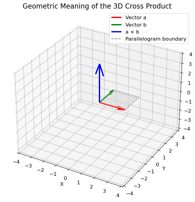
Geometric Interpretation
The definition of the cross product in (6.1) hides some very interesting geometric information about
the direction and
the length of the cross product, which can be explained at hand by the parallelogram spanned by the vectors \(\mathbf{a}\) and \(\mathbf{b}\).

Fig. 6.7 Parallelogram spanned by two vectors \(\mathbf{a}\) and \(\mathbf{b}\).#
Direction
The direction of the cross product \(\mathbf{a} \times \mathbf{b}\) is orthogonal to the parallelogram spanned by the vectors \(\mathbf{a}\) and \(\mathbf{b}\). To proof that \(\mathbf{a} \times \mathbf{b}\) is indeed orthogonal, you can show that the dot product of \(\mathbf{a} \times \mathbf{b}\) and either \(\mathbf{a}\) or \(\mathbf{b}\) is 0:
However, there are two opposite directions that are both orthogonal to \(\mathbf{a}\) and \(\mathbf{b}\). By convention, we follow the right-hand rule where \(\mathbf{a}\) points in the direction of the index finger, \(\mathbf{b}\) points in the direction of the middle finger and \(\mathbf{a} \times \mathbf{b}\) points in the direction of the thumb.

Fig. 6.8 Right-hand rule. Source: https://en.wikipedia.org/wiki/Right-hand_rule#
Length
The magnitude of \(\mathbf{a} \times \mathbf{b}\) equals the area of the parallelogram spanned by the vectors:
where \(\theta\) is the angle between \(\mathbf{a}\) and \(\mathbf{b}\). Intuitively, this means that the more perpendicular the vectors \(\mathbf{a}\) and \(\mathbf{b}\) are, the greater the parallelogram and the greater the magnitude of the cross product! In contrast, the smaller \(\theta\) is, the smaller the magnitude will be. In fact, for parallel lines (when \(\theta\) is \(0^{\circ}\) or \(180^{\circ}\)), the cross product will be 0. This can be easily observed from (6.4).
See the example below for an illustration of these properties. Try to vary
The angle \(\theta\) and observe how it changes the magnitude of the cross product.
Similarly, try to change the length of either \(\mathbf{a}\) or \(\mathbf{b}\) and observe how it changes the magnitude of the cross product.
Try to change the directions of the vectors and see how it affects the direction of the cross product.
def generate_vectors(L_a, L_b, theta_deg):
    """
    Returns two 3D vectors a and b with given magnitudes and angle between them.
    a is aligned with +x axis.
    b lies in x-y plane at the specified angle from a.
    """
    theta = np.radians(theta_deg)

    # Vector a along x-axis
    a = np.array([L_a, 0, 0])

    # Vector b at angle theta in x-y plane
    b = np.array([L_b * np.cos(theta), L_b * np.sin(theta), 0])

    return a, b


# Define two 3D vectors
L_a = 2  # Length
L_b = 2
theta_deg = 90  # angle in degrees

a, b = generate_vectors(L_a, L_b, theta_deg)

# Cross product
c = np.cross(a, b)

# Points for the parallelogram
verts = [[[0, 0, 0], a, a + b, b]]  # list of 4 vertices

fig = plt.figure(figsize=(10, 8))
ax = fig.add_subplot(111, projection="3d")

# Plot vectors a and b
ax.quiver(0, 0, 0, a[0], a[1], a[2], color="red", linewidth=3, label="Vector a")
ax.quiver(0, 0, 0, b[0], b[1], b[2], color="green", linewidth=3, label="Vector b")

# Plot cross-product vector
ax.quiver(0, 0, 0, c[0], c[1], c[2], color="blue", linewidth=3, label="a × b")

# Plot boundary
parallelogram = np.array([[0, 0, 0], a, a + b, b, [0, 0, 0]])
ax.plot(
    parallelogram[:, 0],
    parallelogram[:, 1],
    parallelogram[:, 2],
    color="gray",
    linestyle="--",
    label="Parallelogram boundary",
)

# Fill the parallelogram surface
poly = Poly3DCollection(verts, facecolors="lightgray", alpha=0.5)
ax.add_collection3d(poly)

# Formatting
ax.set_title("Geometric Meaning of the 3D Cross Product", fontsize=16)
ax.set_xlabel("X")
ax.set_ylabel("Y")
ax.set_zlabel("Z")
ax.legend()

# Set equal aspect ratio
max_range = np.array([a, b, c]).max()
for axis in [ax.set_xlim, ax.set_ylim, ax.set_zlim]:
    axis([-max_range, max_range])

plt.show()
Algebraic Properties
Finally, there are also some algebraic properties of the vector cross product that are worth noting:
Anti-commutativity: \(\mathbf{a} \times \mathbf{b} = -(\mathbf{b} \times \mathbf{a})\)
Distributivity: \(\mathbf{a} \times (\mathbf{b} + \mathbf{c}) = \mathbf{a} \times \mathbf{b} + \mathbf{a} \times \mathbf{c}\)
Scalar multiplication \((\lambda \mathbf{a}) \times \mathbf{b} = \lambda (\mathbf{a} \times \mathbf{b})\)
6.3.10. Matrix decompositions#
In linear algebra, a matrix decomposition or matrix factorization is used to split a matrix into a product of other matrices. The goal is to make certain applications of the original matrix easier or more efficient to calculate. As an example, QR decomposition is used to decompose the matrix \(A\) in a linear system of equations \(Ax=b\) into a unitary matrix \(Q\) (or orthogonal if \(A\) has only real elements) and an upper triangular matrix \(R\) such that the original equation can be rewritten to:
Because the inverse of \(Q\) is equal to its transpose. Because \(R\) is triangular, the system is easily solvable without inverting a matrix.
Many more decompositions exist, and a lot of them are listed here. In this section we will only treat the singular value decomposition.
6.3.10.1. Singular value decomposition#
The singular value decomposition (SVD) is applicable to any \(m \times n\) (complex or real) matrix \(A\), and will decompose it as follows:
Where \(U\) is an \(m \times m\) unitary (for complex \(A\)) or orthogonal (for real \(A\)) matrix, \(\Sigma\) is an \(m \times n\) diagonal matrix with the matrix \(A\)’s singular values, and \(V\) is an \(n \times n\) unitary (for complex \(A\)) or orthogonal (for real \(A\)) matrix. See the following figure for a visualization of the resulting matrices and their dimensions.

Fig. 6.9 Matrix dimensions of the singular value decomposition of \(A\).#
A = rng.random((5, 5))

U, S, Vh = np.linalg.svd(A)

np.allclose(U @ np.diag(S) @ Vh, A)
True
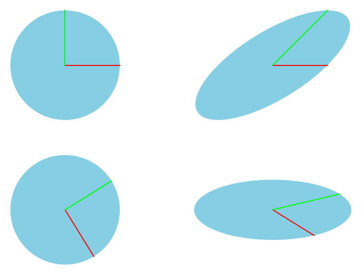
If we regard matrix \(A\) as a linear transformation matrix, the SVD can be geometrically interpreted as a combination of a rotation in \(n\)-dimensional space, a scaling with the singular values along the principal axes of the rotated space (including a scaling by \(0\) for the dimensions that are not included in \(n\)-dimensional space), and a back-rotation in \(m\)-dimensional space.
For the \(2 \times 2\) slanting transformation matrix, defined as:
We can visualize the factors \(U\), \(\Sigma\), and \(V\ConjugateTransposed\) by applying them sequentially to the unit circle, and compare the result to the direct linear transformation using \(A\). Fig. 6.10 is adapted from a similar figure here.

Fig. 6.10 Geometric interpretation of the components that result from the SVD of matrix \(A\).#
We can reconstruct this image as follows:
A = np.array([[1, 1], [0, 1]])

U, S, Vh = np.linalg.svd(A)

x = np.array([[1], [0]])
y = np.array([[0], [1]])
t = np.linspace(0, 2 * np.pi, 101)
xy_unit_circle = np.array([np.cos(t), np.sin(t)])

fig, axs = plt.subplots(2, 2)

for r in axs:
    for e in r:
        e.set_aspect("equal")
        e.set_axis_off()

# Plot normal unit circle
axs[0, 0].plot([0, x[0].item()], [0, x[1].item()], color=(1, 0, 0))
axs[0, 0].plot([0, y[0].item()], [0, y[1].item()], color=(0, 1, 0))
axs[0, 0].add_patch(Polygon(xy_unit_circle.T, ec=None, fc=SAXION_COLS.BLUE))

x = np.array([[1], [0]])
y = np.array([[0], [1]])

# Transform with V^H
x = Vh @ x
y = Vh @ y
xy_unit_circle = Vh @ xy_unit_circle

axs[1, 0].plot([0, x[0].item()], [0, x[1].item()], color=(1, 0, 0))
axs[1, 0].plot([0, y[0].item()], [0, y[1].item()], color=(0, 1, 0))
axs[1, 0].add_patch(Polygon(xy_unit_circle.T, ec=None, fc=SAXION_COLS.BLUE))

# Append transformation with Sigma
x = np.diag(S) @ x
y = np.diag(S) @ y
xy_unit_circle = np.diag(S) @ xy_unit_circle

axs[1, 1].plot([0, x[0].item()], [0, x[1].item()], color=(1, 0, 0))
axs[1, 1].plot([0, y[0].item()], [0, y[1].item()], color=(0, 1, 0))
axs[1, 1].add_patch(Polygon(xy_unit_circle.T, ec=None, fc=SAXION_COLS.BLUE))

# Append transformation with U
x = U @ x
y = U @ y
xy_unit_circle = U @ xy_unit_circle

axs[0, 1].plot([0, x[0].item()], [0, x[1].item()], color=(1, 0, 0))
axs[0, 1].plot([0, y[0].item()], [0, y[1].item()], color=(0, 1, 0))
axs[0, 1].add_patch(Polygon(xy_unit_circle.T, ec=None, fc=SAXION_COLS.BLUE))

plt.show()
The SVD can be used to determine the pseudoinverse of any complex or real matrix \(A\). For matrix \(A\) with SVD \(A=U\Sigma V\ConjugateTransposed\) the pseudoinverse \(A\PseudoInverse\) is found by:
Where the pseudoinverse of \(\Sigma\) is easily determined (because it is diagonal) by taking the reciprocal of all diagonal elements and then taking the transpose.
A = rng.random((5, 8))

A_dagger = np.linalg.pinv(A)

U, S, Vh = np.linalg.svd(A)

# Create an empty array of the correct dimensions as template for S_dagger
S_dagger = np.zeros((8, 5))

# Determine the pseudoinverse of S by taking the element-wise reciprocal of
# the diagonal elements, and filling them in the template we created in the
# previous step.
np.fill_diagonal(S_dagger, np.reciprocal(S))

np.allclose(A_dagger, Vh.conj().T @ S_dagger @ U.conj().T)
True